A Study of TPL in a Multi-Species Population

The original objective of this project was to investigate a possible connection between Taylor’s Power Law (TPL) and Fisher’s \(\alpha\)-diversity metric. It has since evolved into a broader study of how the mean-variance distribution of a particular multi-species population relates to the absolute maximum number of species in a domain. This article summarizes my findings.

import matplotlib.pyplot as plt
import numpy as np
import pandas as pd

from matplotlib.offsetbox import AnchoredText
from scipy import odr
from scipy.interpolate import griddata
from scipy.optimize import newton
from scipy.stats import multivariate_normal

# Plotting config
%matplotlib inline

Domain

Let \(D\) be some finite spatial domain in which a multi-species population exists with unknown distribution. Let \(D\) be divided evenly and completely into \(Q\) total bins. We can think of \(Q\) as our “domain resolution”.

Let \(S\) be the absolute maximum number of species found in \(D\). Although \(S\) is unknown, we know that it is finite because \(D\) is finite. We would like to estimate this number.

If we take \(1 \leq q \leq Q\) samples from the domain and count up the number of individuals of each species in each bin, then we can create a bin-count array for each encountered species. The array for a species would take the form \(X=\{x_0, x_1, ... x_{q-1}\}\). Whenever we speak of mean \(M\) and variance \(V\) in this document, we’re referring to the mean and variance of \(X\) for some \(q\).

The \(\Phi\) function

Given some \(Q\), let \(\Phi(M,V)\) be a function that returns the expected number of zeros values in any bin-count array that satisfies \(M\) and \(V\). In other words, \(\Phi\) tells us how may \(x_i\) items in \(X=\{x_0, x_1, ... x_{Q-1}\}\) we can expect to be zero when the mean and variance of \(X\) are \(M\) and \(V\) respectively.

\(\Phi\) is useful because it can be used to compute \(\lambda_q (M,V)\), the probability that a species with a particular \(M\) and \(V\) can remain unobserved after \(q\) samples.

For example, if we are working in a domain with \(Q=10\) total bins, and a particular mean and variance yield \(\Phi=5\) expected zeros, then the probability that a species will remain unobserved after \(q=3\) samples is:

Because of the combinatorics involved, \(\Phi\) can only be computed deterministically for small \(Q\) and small \(N=\sum X\). As either \(Q\) or \(N\) grow, the number of possible combinations of \(X\) grows exponentially. For the purpose of this study, I’ve produced two lookup matrices for \(\Phi\) using brute-force methods. The first is for \(Q=50\) and the second for \(Q=100\). In both cases, \(N\) is bounded by \(1\leq N \leq 100\).

def build_phi(dfZ, Q_sup, stat='max', V_scale=10):
    assert stat in ('min', 'max', 'mean', 'count')

    # Determine ranges and shape of output
    N_rng = np.arange(dfZ['N'].min(), dfZ['N'].max() + 1)
    assert N_rng[0] > 0
    M_rng = N_rng / Q_sup
    V_min = dfZ['V'][dfZ['V'] > 0].min()  # remove zero variance
    V_rng = np.linspace(V_min, dfZ['V'].max(), len(N_rng) * V_scale)
    shape = (len(M_rng), len(V_rng))

    # This matrix counts number of data point in each 2d bin
    bin_counts, _, _ = np.histogram2d(
        dfZ['M'], dfZ['V'],
        bins=shape,
        range=[
            [M_rng[0], M_rng[-1]],
            [V_rng[0], V_rng[-1]]],
        density=False,
        )
    
    # This matrix sums up the given statistic for each 2d bin
    Phi, _, _ = np.histogram2d(
        dfZ['M'], dfZ['V'],
        weights=dfZ[stat],
        bins=shape,
        range=[
            [M_rng[0], M_rng[-1]],
            [V_rng[0], V_rng[-1]]],
        density=False,
        )

    # Divide the stat sums by their corresponding counts
    Phi[bin_counts>0] /= bin_counts[bin_counts>0]
    
    # Round up or down for "max" and "min" stats
    if stat == 'max':
        Phi = np.ceil(Phi).astype(int)
    elif stat == 'min':
        Phi = np.floor(Phi).astype(int)

    return Phi, N_rng, M_rng, V_rng


# Phi for Q=50 and 1<=N<=100
dfZ_a = pd.read_hdf('zeros_q50_n100.h5', 'df')
Phi_a, N_rng_a, M_rng_a, V_rng_a = build_phi(dfZ_a, 50, 'mean')

# Phi for Q=100 and 1<=N<=100
dfZ_b = pd.read_hdf('zeros_q100_n100.h5', 'df')
Phi_b, N_rngb, M_rng_b, V_rng_b = build_phi(dfZ_b, 100, 'mean')

# Plot
fig, ax = plt.subplots(1, 2, sharey=False)
fig.set_figwidth(12)
ax[0].pcolor(M_rng_a, V_rng_a, Phi_a.T, cmap='magma')
ax[0].set_title('$\Phi$ for $Q=50$')
ax[0].set_xlabel('Mean')
ax[0].set_ylabel('Variance')
ax[1].pcolor(M_rng_b, V_rng_b, Phi_b.T, cmap='magma')
ax[1].set_title('$\Phi$ for $Q=100$')
ax[1].set_xlabel('Mean')
ax[1].set_ylabel('Variance');

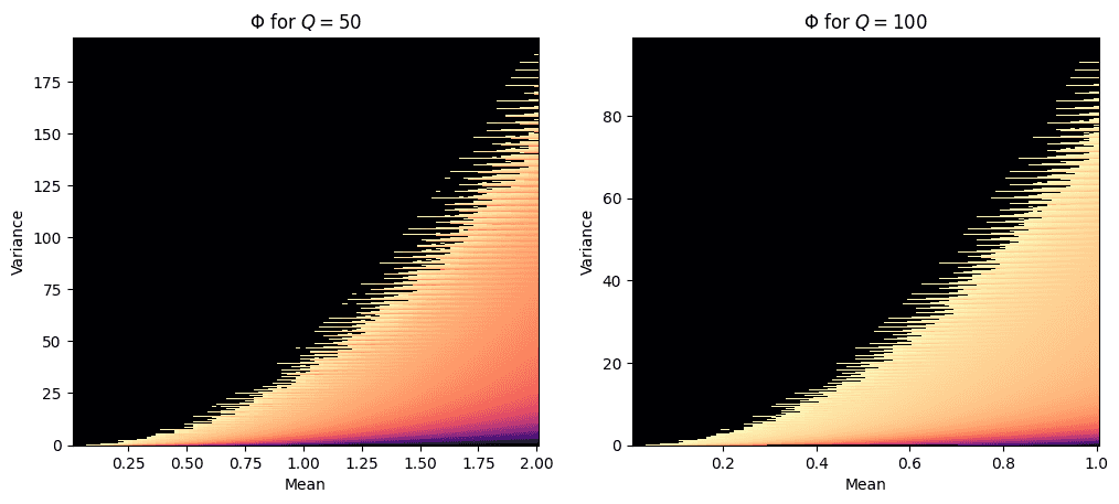
The two heatmaps above show \(\Phi\) for \(Q=50\) and \(Q=100\). The brighter the color, the greater the expected number of zeros for that corresponding \(M\) and \(V\). Notice how \(\Phi\) has a fractal boundary of sorts when \(V\) is maximized for a given \(M\). This boundary is where we expected to find the highest number of zeros. On the other hand, when \(V\) is minimized for a given \(M\), we see few zeros.

Random populations

def orth_fit(x, y):
    odr_obj = odr.ODR(odr.Data(x, y), odr.unilinear)
    output = odr_obj.run()
    return output.beta


def calc_rho(pdf, Phi, Q, Q_sup):

    pdf = pdf.T.copy()
    pdf[Phi<=0] = 0  # get rid of impossible values
    pdf /= pdf.sum()
    
    # For each (M,V), if Phi(M,V) zeros are expected (of Q_sup bins),
    # then to the probability of getting Q zeros in a row at the beginning
    # is this product.
    lam = 1
    for i in range(Q):
        rem = Phi-i
        rem[rem<0] = 0
        lam *= rem / (Q_sup-i)

    rho = (pdf * lam).sum()

    return rho


class Population:
    
    def __init__(self, path, Q_sup=None, N_sup=None, S_sup=None, name=None):
        
        self.Q_sup = 50 if Q_sup is None else Q_sup
        self.N_sup = 100 if N_sup is None else N_sup
        self.S_sup = 200 if S_sup is None else S_sup
        self.name = 'Population' if name is None else name
        self.Q_cols = np.array([f'Q{i}' for i in range(self.Q_sup)])  # column names

        self.df_path = path
        self.df = pd.read_hdf(self.df_path, 'df')
        
        self.dfZ_path = f'zeros_q{self.Q_sup}_n{self.N_sup}.h5'
        self.dfZ = pd.read_hdf(self.dfZ_path, 'df')

        self.Phi, self.N_rng, self.M_rng, self.V_rng = build_phi(self.dfZ, self.Q_sup, 'max')
        self.pdf_true = self.get_pdf(self.df['M'].to_numpy(), self.df['V'].to_numpy())

        self.dfS = self.simulate()
        
    def get_pdf(self, M, V, allow_singular=False):

        # Fit a 2D normal distribution to the data (in log space)
        M_ln = np.log(M)
        V_ln = np.log(V)
        rv = multivariate_normal(
            mean=[np.mean(M_ln), np.mean(V_ln)],
            cov=np.cov(M_ln, V_ln),
            allow_singular=allow_singular,
            )
        Xm, Ym = np.meshgrid(self.M_rng, self.V_rng)
        pos = np.dstack((Xm, Ym))
        pdf = rv.pdf(np.log(pos))
        
        pdf /= pdf.sum()
        pdf[np.isclose(pdf, 0)] = 0
        pdf /= pdf.sum()
        
        return pdf

    def simulate(self, shuffle=False):

        # Select bin data
        Q_cols = self.Q_cols.copy()
        if shuffle:
            np.random.shuffle(Q_cols)
        df = self.df[Q_cols].copy()

        # Count unique species across entire domain, starting from left bin
        dfS = pd.DataFrame({
            'Q': range(1, len(Q_cols)+1),
            'S': np.count_nonzero(
                np.cumsum(df, axis=1),
                axis=0),
            })

        for i in range(len(Q_cols)):
            cols = Q_cols[:i+1]
            _df = df[cols].copy()
            _N = np.sum(_df, axis=1)
            _M = np.mean(_df, axis=1)
            _V = np.var(_df, axis=1)
            _df['N'] = _N
            _df['M'] = _M
            _df['V'] = _V

            # Discard species with zero mean or variance
            _df = _df[(_df['M'] > 0) & (_df['V'] > 0)]

            tpl_b, tpl_a, rho = np.nan, np.nan, np.nan
            if len(_df.index) > 1:
                M_ln = np.log(_df['M'].to_numpy())
                V_ln = np.log(_df['V'].to_numpy())
                tpl_b, tpl_a_ln = orth_fit(M_ln, V_ln)
                tpl_a = np.exp(tpl_a_ln)

                # Note: using true PDF
                pdf = self.pdf_true

                rho = calc_rho(pdf, self.Phi, i+1, self.Q_sup)

            dfS.loc[i, ['b', 'a', 'rho']] = tpl_b, tpl_a, rho
            
        return dfS
        

# Population datasets
populations = [
    Population('pop_4_q50_n100_s200.h5', Q_sup=50, name='A1'),
    Population('pop_5_q50_n100_s200.h5', Q_sup=50, name='A2'),
    Population('pop_6_q50_n100_s200.h5', Q_sup=50, name='A3'),
    Population('pop_1_q100_n100_s200.h5', Q_sup=100, name='B1'),
    Population('pop_2_q100_n100_s200.h5', Q_sup=100, name='B2'),
    Population('pop_3_q100_n100_s200.h5', Q_sup=100, name='B3'),
    ]


def scatter_plot(pop, ax=None):
    if ax is None:
        fig, ax = plt.subplots(1, 1)

    M = pop.df['M']
    V = pop.df['V']
    M_ln = np.log(M)
    V_ln = np.log(V)
    N_rng = pop.N_rng
    M_rng = pop.M_rng

    ax.scatter(M, V, 1, marker='+')
    ax.set_xscale('log')
    ax.set_yscale('log')
    ax.set_title(f'Population {pop.name}')
    # ax.set_xlabel('M')
    # ax.set_ylabel('V')

    V_bounds = np.zeros((len(M_rng), 2))
    for i, n in enumerate(N_rng):
        s = np.zeros(pop.Q_sup)
        s[0] = n
        max_ = s.var()

        quo, mod = np.divmod(n, pop.Q_sup)
        s[:mod] = quo + 1
        s[mod:] = quo
        assert s.sum() == n
        min_ = s.var()
        V_bounds[i] = (min_, max_)

    ax.plot(M_rng, V_bounds[:, 0], '--', color='tab:gray')
    ax.plot(M_rng, V_bounds[:, 1], '--', color='tab:gray')

    est_b, est_a_ln = orth_fit(M_ln, V_ln)
    est_a = np.exp(est_a_ln)

    V_tpl = np.exp(np.log(est_a)+est_b*np.log(M))
    ax.plot(M, V_tpl, 'b-', linewidth=1)

    # ax = plt.gca()
    tpl_text = '$b = %.2f$   $a = %.2f$' % (est_b, est_a)
    at = AnchoredText(
        tpl_text, loc='upper left', prop=dict(size=8), frameon=True)
    at.patch.set_boxstyle('round, pad=0., rounding_size=0.2')
    ax.add_artist(at)


# Plot
fig, ax = plt.subplots(2, 3, sharey=True)
fig.set_figheight(8)
fig.set_figwidth(16)
plt.subplots_adjust(hspace=0.4)
for i, pop in enumerate(populations):
    row = int(i/ax.shape[1])
    col = i % ax.shape[1]
    scatter_plot(pop, ax[row][col])

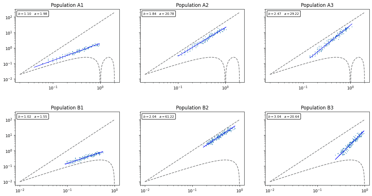
I’ve generated 6 random multi-species populations. The first 3 (labels starting with A) assume \(Q=50\). The second 3 (labels starting with B) assume \(Q=100\). In all cases, the absolute maximum number of species is \(S=200\). As you can see, each population has a slightly different distribution in \(M\times V\) space and demonstrates its own TPL.

The question I’m interested in: How do the distributions of these different populations affect the expected species count \(s_q\) at iteration \(q\) as \(q\rightarrow Q\)? In other words, as we iteratively count up all individuals in the domain by increasing the bin count, how quickly or slowly do we find new species?

It turns out that when a population consists mainly of highly aggregated species, then it will take longer for \(s_q \rightarrow S\) than if the distributions are more uniform. This makes intuitive sense, as uniform species are spread out more evenly among the bins so they will be discovered quickly.

As an illustration, let’s plot out \(s_q\) against \(q\) for two populations with very distinct distributions.

for i in [3, 4]:
    pop = populations[i]
    plt.plot(pop.dfS['Q'], pop.dfS['S'], label=f'Population {pop.name}')
plt.legend()
plt.xlabel('$q$')
plt.ylabel('$s_q$')
plt.title('Convergence of $s_q \\rightarrow S$ as $q \\rightarrow Q$');

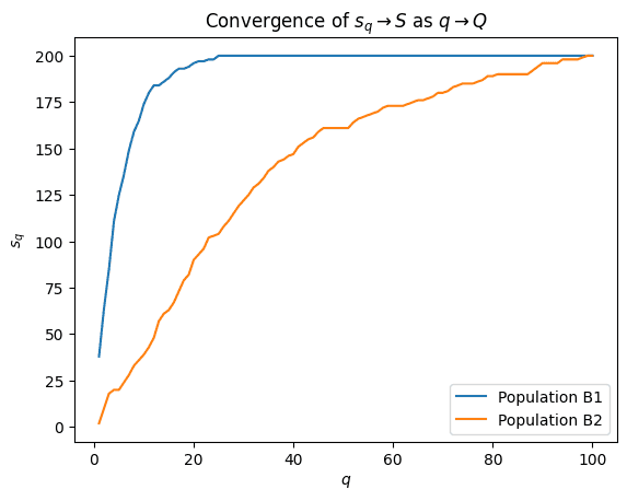
Notice the clear difference in shape between the convergence lines of populations B1 and B2. Population B1 has less variance than B2 (therefore more uniform), so we can expect the various species to be discovered at earlier iterations \(q\).

So, in theory, if you know how much as been sampled and you have a good idea as to the degree of aggregation in the population, then you should be able to place an estimate on the absolute total number of species.

Estimating \(S\)

Let \(\rho_{q,i}\) be the probability of failing to observe the \(i\)-th species after \(q\) samples. Then \(1-\rho_{q,i}\) is the probability of having observed the \(i\)-th species after \(q\) samples. It follows that \(s_q\), the number of species observed after \(q\) samples, can be written thus:

Recall from before that the probability that a species with a given \(M\) and \(V\) will remain unobserved after \(q\) samples is given by the function \(\lambda_q\) (derived from \(\Phi\)). If the \(i\)-th species has mean \(M_i\) and variance \(V_i\), then it follows that:

If \(f\) is the true probability distribution function (PDF) of the population in \(M\times V\) space, then we can write the expected value of \(\rho_{q,i}\) for the entire population as:

We are essentially piece-wise multipying \(f\) with \(\lambda_q\) across the entire \(M\times V\) domain. Plugging \(\rho_q\) back into the original equation yields:

Rewritten we have a formula for estimating \(S\) given \(s_q\) and \(\rho_q\) (which depends on \(f\) and \(\Phi\)):

The key concept is the estimation of \(\rho_q\), which can be conveniently visualized by superimposing \(f\) onto \(\lambda_q\) for a given \(q\).

lam = 1
q = 20
for i in range(q):
    rem = Phi_b-i
    rem[rem<0] = 0
    lam *= rem / (pop.Q_sup-i)

pop = populations[4]  # B2
fig, ax = plt.subplots(1, 3, sharey=True)
fig.set_figwidth(16)

ax[0].pcolor(M_rng_b, V_rng_b, pop.pdf_true, cmap='magma')
ax[0].set_title('PDF')
ax[0].set_ylabel('V')
ax[0].set_xlabel('M')
ax[1].pcolor(M_rng_b, V_rng_b, lam.T, cmap='magma')
ax[1].set_title('$\lambda_{%i}$' % q)
ax[1].set_xlabel('M')
ax[2].pcolor(M_rng_b, V_rng_b, pop.pdf_true * lam.T, cmap='magma')
ax[2].set_title('PDF$\cdot\lambda_{%i}$' % q)
ax[2].set_xlabel('M');

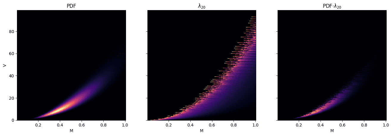
The first plot is the PDF of Population B2 in \(M\times V\) space. The second plot is \(\lambda_q\) at \(q=20\) which tells us where we’re most likely to have unobserved species after 20 samples, irrespective of PDF. The third plot shows the two functions multiplied together; this tells us where we’re most likely to have unobserved species given the PDF.

Results

Now let’s test the theory for each of the 6 populations.

def sim_plot(pop, ax=None, shuffle=False):
    if ax is None:
        fig, ax = plt.subplots(1, 1)

    dfS = pop.simulate(shuffle=True) if shuffle else pop.dfS
    ax.plot(dfS['Q'], dfS['S'])
    ax.plot(dfS['Q'], pop.S_sup * (1-dfS['rho']))
    ax.plot(dfS['Q'], dfS['S'] / (1-dfS['rho']))
    ax.set_title(f'Population {pop.name}')
    ax.set_xlabel('q')

# Cumulative species count
fig, ax = plt.subplots(2, 3, sharey=True)
fig.set_figheight(8)
fig.set_figwidth(16)
plt.subplots_adjust(hspace=0.4)
for i, pop in enumerate(populations):
    row = int(i/ax.shape[1])
    col = i % ax.shape[1]
    sim_plot(pop, ax=ax[row][col], shuffle=False)
ax[0][0].set_ylabel('species count')
ax[1][0].set_ylabel('species count');

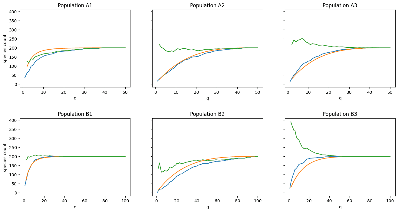
How to interpret these plots:

• The blue line is the observed number of species \(s_q\) as \(q\rightarrow Q\).
• The green line is our estimate of \(S\) given \(s_q\) (we expect this line to approach \(S=200\) in all cases).
• The orange curve is what we expect our species curve to look like given \(\lambda_q\) and prior knowledge of \(S\). The closer the blue and orange lines are together, the better our estimate of \(S\) will be (green line).

Visual inspection yields mixed results:

• Populations A2, A3, and B1 show excellent alignment
• Populations A1 and B2 show “okay” alignment
• Population B3 shows very poor alignment

Discussion

First of all, the procedure for estimating \(S\) demonstrated above has one enormous shortcoming: it requires prior knowledge of \(f\), the population’s PDF in \(M\times V\) space. While it may be possible in some cases to estimate \(f\) using available data, I have observed that the closer \(f\) gets to the fractal boundary inherent in \(M\times V\) space, the less reliable it becomes. This is likely due to the fact that as \(q\rightarrow Q\), we’re most likely to observe species with higher mean and lower variance first, then work our way to the fractal boundary. This phenomenon ends up distorting our estimate of \(f\).

Secondly, it can be seen clearly from the results that the procedure is not fool-proof. In particular, predictions for Populations A1 and B2 were farther off than I’d like, while B3 was way off. My hunch is that these outliers are due to a failure to take into account the higher-order moments of \(X\), in particular skew. If this is true, then the solution is to include skew in all estimations. In other words, I must extend both \(f(M,V)\) and \(\Phi(M,V)\) into \(f(M,V,S)\) and \(\Phi(M,V,S)\). Probably doable, but it obviously adds complexity.

It may be possible to side-step both issues by applying a non-linear machine learning algorithm (e.g. neural network) to the available data. There is clearly a strong connection between the population distribution, \(S\), and \(Q\), but the fractal nature of \(M\times V\) space (or \(M\times V\times S\) space) makes computations difficult. Machine learning is sometimes quite good at teasing apart these kinds of relationships. But… it wouldn’t be an analytic solution like I wanted.

Now let’s consider the \(\Phi\) function. As mentioned before, I use brute-force methods to estimate \(\Phi\) for a given \(Q\) and max \(N\). The procedures outlined in this document won’t be scalable until a better way is found to either compute or estimate \(\Phi\) for any \(Q\) and \(N\). I suspect that the fractal/ combinatorial nature of \(\Phi\) prevents it from being computed exactly in an efficient way. But it does seem behave in a somewhat predictable way, so perhaps it can be suitably estimated in a simple way.

Possible lead?

Is it possible to somehow remove the need for prior knowledge of \(f\)? I don’t know, but here’s a possible lead.

Given:

• Let \(f\) be the PDF of all species in \(\ln (M) \times \ln (V)\) space after all \(Q\) samples have been taken.
• Let \(g\) be the PDF of observed species after \(q\) samples taken.
• Let \(h\) be the PDF of unobserved species after \(q\) samples taken.

It follows that \(g\) is proportional to \(f \cdot (1-\lambda_q)\) and \(h\) is proportional to \(f \cdot \lambda_q\). Alternatively, \(g = c_1 f \cdot (1-\lambda_q)\) and \(h = c_2 f \cdot \lambda_q\) for some scaling factors \(c_1 \geq 1\) and \(c_2 \geq 1\). Note that if \(f \cdot (1-\lambda_q) = 0\) then \(f=h\). Likewise, if \(f \cdot \lambda_q = 0\) then \(f=g\) (this can probably be formulated better).

We can write \(f\) in terms of \(g\) and \(h\) like so:

If \(s_q\) is the number of species observed after \(q\) samples, I believe it’s possible to show that \(f\) is a weighted average of \(g\) and \(h\) with:

Thus we have a relation between \(f\) and \(S\) given \(g\) and \(s_q\):

Here we have a relation between two unknowns. There’s not much more to be done without additional traction. Perhaps this can be formulated as an optimization problem in which we simultaneously solve for \(f\) and \(S\), but I don’t know what the objective function might be. I think more assumptions about the nature of \(f\), \(g\), and/ or \(h\) are needed. It would be nice to be able to use TPL, but unfortunately TPL’s \(b\) and \(a\) do not necessarily remain constant as \(q \rightarrow Q\).

Here’s a thought experiment. Let’s say you’ve taken \(q=1\) sample of \(Q=10\) total samples and it yielded \(s_1=3\) species. According to the relation above, there should be a PDF \(f\) corresponding to any \(S\geq 3\). For example, it’s entirely possible that the total species count is the same as your first sample, \(S=s_1=3\). In which case I’d assume that the 3 species are distributed in a uniform way; it seems unlikely that they are highly aggregated and you just got all 3 in your first sample by luck. It’s also entirely possible that \(S\) is very large, but keep in mind that the larger \(S\) gets, the more it becomes a fluke that you didn’t get more than 3 in your first sample. So it appears that \(S\) is bounded, at least in a probabilistic sense. As \(q \rightarrow Q\), I’d expect that bound to become tighter and tighter. A possible upper bound for \(S\) might be \((s_q \cdot Q) / q\).

So, given our first sample, right off the bat there are certain \((f, S)\) pairings that become unlikely. The task becomes how to find the “best” \(f\) that fits the known data while minimizing outliers (error). It might be that the “best” \(f\) is actually just \(g\) (PDF of observed species), but I’m unsure.

References

1. Taylor, R. A. (2019). Taylor’s power law: order and pattern in nature. Academic Press.
2. Fisher, R. A., Corbet, A. S., & Williams, C. B. (1943). The relation between the number of species and the number of individuals in a random sample of an animal population. The Journal of Animal Ecology, 42-58.