In a previous post I talked about the Dynamic Mode Decomposition (DMD) and how to implement it in Python. I mentioned near the end of that post that there exist a number of variants of the DMD. Some variants attempt to resolve certain shortcomings of the DMD; others attempt to extend the core concepts in interesting ways. One such variant is the sparsity-promoting DMD (spDMD) developed by Jovanović et al.
The spDMD is mostly motivated by the question of how to find the best modes for a system. It is a non-trivial question. Typically, it is necessary for a human expert to be “in-the-loop”, making a judgment on which DMD modes to use. This is great (ideal even) when the application is just a one-time analysis. But what about when the application of the DMD needs to be automated?
There are several approaches to automating rank-reduction in a principled manner. Previously, I posted on an approach called the optimal SVHT. It is an easy to implement method that computes an optimal cutoff value for truncating singular values. It can applied to any SVD-based method — including the DMD.
The spDMD is another approach that applies specifically to the DMD. It uses some clever optimization tricks to try to reconstruct the original data with as few DMD modes as possible. The phrase “sparsity-promoting” in the method’s name refers to the concept of preferring DMD solutions with sparse sets of nonzero modes.
Here I introduce the core concepts of the spDMD and provide a rudimentary implementation in Python.
We Start with the DMD
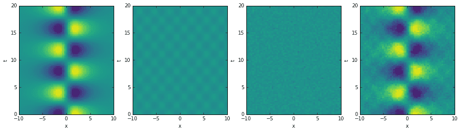
As per usual, let’s start the investigation by constructing a toy example. Here is code for building a relatively simple data set consisting of one strong mode, one weak mode, and some normally distributed noise. The resulting data is centered around the origin, so we won’t worry about removing the mean and variance (normalizing the data). From left to right, the four images below show each mode matrix, the noise matrix, and the final summation. The summed data matrix is what we’ll pass into the DMD algorithm.
import numpy as npimport matplotlib as mplimport matplotlib.pyplot as pltfrom mpl_toolkits.mplot3d import Axes3Dfrom numpy import dot, multiply, diagfrom numpy.linalg import inv, eig, pinv, norm, solve, choleskyfrom scipy.linalg import svd, svdvalsfrom scipy.sparse import csc_matrix as sparsefrom scipy.sparse import vstack as spvstackfrom scipy.sparse import hstack as sphstackfrom scipy.sparse.linalg import spsolve# define time and space domainsx = np.linspace(-10, 10, 60)t = np.linspace(0, 20, 80)Xm,Tm = np.meshgrid(x, t)# create dataD1 = 5 * (1/np.cosh(Xm/2)) * np.tanh(Xm/2) * np.exp((0.8j)*Tm) # strong primary modeD2 = 0.2 * np.sin(2 * Xm) * np.exp(2j * Tm) # weak secondary modeD3 = 0.1 * np.random.randn(*Xm.shape) # noiseD = (D1 + D2 + D3).T
Now we call the DMD routine to find the DMD modes \(\Phi\) and eigenvalues \(\mu\). The DMD code listed below is condensed, so see my DMD post if you’re curious for an explanation. Note that we’re rank-reducing a bit with \(r=30\). Ideally, we’d rank-reduce all the way up to \(r=2\) (two modes were used to construct the data). However, the idea here is to test out the rank-reducing capabilities of the spDMD — so we’ll leave a healthy number of garbage modes.
def dmd(X, Y, truncate=None):U2,Sig2,Vh2 = svd(X, False) # SVD of input matrixr = len(Sig2) if truncate is None else truncate # rank truncationU = U2[:,:r]Sig = diag(Sig2)[:r,:r]V = Vh2.conj().T[:,:r]Atil = dot(dot(dot(U.conj().T, Y), V), inv(Sig)) # build A tildemu,W = eig(Atil)Phi = dot(dot(dot(Y, V), inv(Sig)), W) # build DMD modesreturn mu, Phi# extract input-output matricesX = D[:,:-1]Y = D[:,1:]# do dmdr = 30 # new rankmu,Phi = dmd(X, Y, r)
The \(b\) Vector
The next step in the DMD work-flow is to reconstruct a matrix corresponding to the time evolution of the system. Specifically, we want to find \(\Psi\) such that
Normally when computing the DMD, we’d simply use the system’s initial conditions \(x_0\) to create a time evolution matrix. I have used the following, verbose method to build \(\Psi\) in the past.
# compute time evolution (verbose way)b = dot(pinv(Phi), X[:,0])Psi = np.zeros([r, len(t)], dtype='complex')dt = t[2] - t[1]for i,_t in enumerate(t):Psi[:,i] = multiply(np.power(mu, _t/dt), b)
But there’s a more concise method to calculate \(\Psi\). We can use a Vandermonde matrix to replace the for loop and then do a simple product. The product can be written analytically like so:
where \(V_\mu\) is the Vandermonde matrix, \(\text{diag}\) is the operation that converts a vector into a diagonal matrix (and vice versa), and \(\dagger\) is the Moore-Penrose pseudo-inverse of matrix.
# compute time evolution (concise way)b = dot(pinv(Phi), X[:,0])Vand = np.vander(mu, len(t), True)Psi = (Vand.T * b).T # equivalently, Psi = dot(diag(b), Vand)
Then the DMD reconstruction in Python would become
D_dmd = dot(Phi, Psi)
Now here’s the critical insight: we’re not restricted to using \(b=\Phi^\dagger x_0\). We could potentially choose \(b\) to be a vector whose corresponding time evolution matches the original data even better (i.e., minimizes the error). Let’s investigate.
Basically, we want to find a solution to the optimization problem
where \(X\) is the original data matrix and \(D_b=\text{diag}\{b\}\) for a given \(b\) vector. Using a clever combination of matrix trace properties, we can rewrite the objective function \(J(b)\) as
where
An asterisk denotes the complex conjugate transpose, an overline denotes the complex conjugate, and \(\circ\) is element-wise multiplication. Refer to the derivations given in Jovanović et al. for a more complete explanation. Just note that their objective function is derived from the standard DMD (using projected DMD modes). Ours is derived from the exact DMD. See Tu et al. or my DMD post for more information on the distinction between exact and projected.
# vars for the objective functionU,sv,Vh = svd(D, False)Vand = np.vander(mu, len(t), True)P = multiply(dot(Phi.conj().T, Phi), np.conj(dot(Vand, Vand.conj().T)))q = np.conj(diag(dot(dot(Vand, (dot(dot(U, diag(sv)), Vh)).conj().T), Phi)))s = norm(diag(sv), ord='fro')**2
The objective function is minimized where its gradient is zero. The solution can be determined analytically:
Finding the optimal \(b\) vector for the DMD in Python is just as easy.
# the optimal solutionb_opt = solve(P, q)
Promoting Sparsity in \(b_\text{optimal}\)
Finding \(b_\text{optimal}\) for our basic rank-reduced DMD is just the beginning. What if we could efficiently find \(b_\text{optimal}\) for all combinations of DMD modes? We could then select the solution that exhibits the best balance of accuracy and sparsity. However, when the rank of our DMD is very large, this task is infeasible — the number of combinations is enormous. But perhaps there’s an optimization algorithm that could find it.
The spDMD incorporates the alternating direction method of multipliers (ADMM) algorithm to search for candidate \(b\) vectors that satisfy both of two conditions: they minimize the objective function \(J(b)\) and they are sparse (few nonzero entries). Specifically, it allows us to solve the optimization problem
Basically, we are optimizing the same problem as before, but with an \(L^1\) penalty (related post: Compressed Sensing in Python). The purpose of the penalty is to discourage non-sparse \(b_\text{optimal}\) vectors. The \(\gamma\) value reflects our emphasis on sparsity. In the code below we use the ADMM (code listed at the end of post) to test a range of \(\gamma\) values to see how they affect the resulting \(b_\text{optimal}\) vectors.
# find optimum solutionsgamma_vec = np.logspace(np.log10(0.05), np.log10(200), 150)answer = admm_for_dmd(P, q, s, gamma_vec)
The spDMD is complete. Now we must analyze the information it yielded. Keep in mind that we are mostly interested in understanding how to gain as much accuracy as we can with as few DMD modes as possible. Take a look at the admm_for_dmd implementation in the following section to see what the return variable looks like.
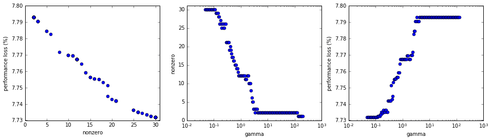
First thing we should do is look to see how the different gamma values relate to the number of nonzero elements in \(b\) and overall performance. In the plots below, the “nonzero” axes reflect the number of nonzero modes and “performance loss” is a normalized indication of the overall model error resulting from the use of \(b_\text{optimal}\). Of course, “gamma” is the \(\gamma\) value.
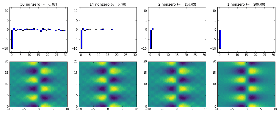
We can also take a look at the different \(b_\text{optimal}\) vectors returned by the ADMM routine. The next set of plots show four \(b_\text{optimal}\) vectors with varying sparsity. Below each of them is the resulting DMD reconstruction. The first three reconstructions are mostly indistinguishable at this resolution, but the fourth is very clearly a 1-mode reconstruction. At higher resolutions the first three are more distinguishable due to their different noise levels.
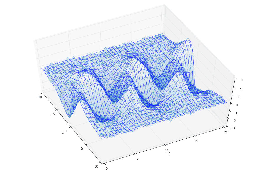
Finally, for some variety, here’s a 3D version of the data. The dotted surface represents the original data (two modes plus noise), while the smooth grid of blue lines represents the 1-mode reconstruction corresponding to a large \(\gamma\) value.
ADMM
The ADMM is very advanced and well beyond the scope of this short post. Suffice it to say that it is very generalizable and can be applied in many contexts; the spDMD is but one of its many applications.
Here I list the code for the admm_for_dmd method used earlier. It is a direct Python translation of the dmdsp MATLAB function used by Jovanović et al. Of course, it is not optimized for speed and is highly specialized to the spDMD problem. Furthermore, it has only been tested with the toy problem above. Perhaps in a future post I’ll tackle the problem of making the code production-quality.
def admm_for_dmd(P, q, s, gamma_vec, rho=1, maxiter=10000, eps_abs=1e-6, eps_rel=1e-4):# blank return valueanswer = type('ADMMAnswer', (object,), {})()# check input varsP = np.squeeze(P)q = np.squeeze(q)[:,np.newaxis]gamma_vec = np.squeeze(gamma_vec)if P.ndim != 2:raise ValueError('invalid P')if q.ndim != 2:raise ValueError('invalid q')if gamma_vec.ndim != 1:raise ValueError('invalid gamma_vec')# number of optimization variablesn = len(q)# identity matrixI = np.eye(n)# allocate memory for gamma-dependent output variablesanswer.gamma = gamma_vecanswer.Nz = np.zeros([len(gamma_vec),]) # number of non-zero amplitudesanswer.Jsp = np.zeros([len(gamma_vec),]) # square of Frobenius norm (before polishing)answer.Jpol = np.zeros([len(gamma_vec),]) # square of Frobenius norm (after polishing)answer.Ploss = np.zeros([len(gamma_vec),]) # optimal performance loss (after polishing)answer.xsp = np.zeros([n, len(gamma_vec)], dtype='complex') # vector of amplitudes (before polishing)answer.xpol = np.zeros([n, len(gamma_vec)], dtype='complex') # vector of amplitudes (after polishing)# Cholesky factorization of matrix P + (rho/2)*IPrho = P + (rho/2) * IPlow = cholesky(Prho)Plow_star = Plow.conj().T# sparse P (for KKT system)Psparse = sparse(P)for i,gamma in enumerate(gamma_vec):# initial conditionsy = np.zeros([n, 1], dtype='complex') # Lagrange multiplierz = np.zeros([n, 1], dtype='complex') # copy of x# Use ADMM to solve the gamma-parameterized problemfor step in range(maxiter):# x-minimization stepu = z - (1/rho) * y# x = solve((P + (rho/2) * I), (q + rho * u))xnew = solve(Plow_star, solve(Plow, q + (rho/2) * u))# z-minimization stepa = (gamma/rho) * np.ones([n, 1])v = xnew + (1/rho) * y# soft-thresholding of vznew = multiply(multiply(np.divide(1 - a, np.abs(v)), v), (np.abs(v) > a))# primal and dual residualsres_prim = norm(xnew - znew, 2)res_dual = rho * norm(znew - z, 2)# Lagrange multiplier update stepy += rho * (xnew - znew)# stopping criteriaeps_prim = np.sqrt(n) * eps_abs + eps_rel * np.max([norm(xnew, 2), norm(znew, 2)])eps_dual = np.sqrt(n) * eps_abs + eps_rel * norm(y, 2)if (res_prim < eps_prim) and (res_dual < eps_dual):breakelse:z = znew# record output dataanswer.xsp[:,i] = z.squeeze() # vector of amplitudesanswer.Nz[i] = np.count_nonzero(answer.xsp[:,i]) # number of non-zero amplitudesanswer.Jsp[i] = (np.real(dot(dot(z.conj().T, P), z))- 2 * np.real(dot(q.conj().T, z))+ s) # Frobenius norm (before polishing)# polishing of the nonzero amplitudes# form the constraint matrix E for E^T x = 0ind_zero = np.flatnonzero(np.abs(z) < 1e-12) # find indices of zero elements of zm = len(ind_zero) # number of zero elementsif m > 0:# form KKT system for the optimality conditionsE = I[:,ind_zero]E = sparse(E, dtype='complex')KKT = spvstack([sphstack([Psparse, E], format='csc'),sphstack([E.conj().T, sparse((m, m), dtype='complex')], format='csc'),], format='csc')rhs = np.vstack([q, np.zeros([m, 1], dtype='complex')]) # stack vertically# solve KKT systemsol = spsolve(KKT, rhs)else:sol = solve(P, q)# vector of polished (optimal) amplitudesxpol = sol[:n]# record output dataanswer.xpol[:,i] = xpol.squeeze()# polished (optimal) least-squares residualanswer.Jpol[i] = (np.real(dot(dot(xpol.conj().T, P), xpol))- 2 * np.real(dot(q.conj().T, xpol))+ s)# polished (optimal) performance lossanswer.Ploss[i] = 100 * np.sqrt(answer.Jpol[i]/s)print(i)return answer
References
- Jovanović, Mihailo R., Peter J. Schmid, and Joseph W. Nichols. “Sparsity-promoting dynamic mode decomposition.” Physics of Fluids (1994-present) 26.2 (2014): 024103.
- http://people.ece.umn.edu/users/mihailo/software/dmdsp/
- Tu, Jonathan H., et al. “On dynamic mode decomposition: theory and applications.” arXiv preprint arXiv:1312.0041 (2013).
- Boyd, Stephen, et al. “Distributed optimization and statistical learning via the alternating direction method of multipliers.” Foundations and Trends® in Machine Learning 3.1 (2011): 1-122.
- http://stanford.edu/~boyd/admm.html
- Wikipedia contributors. “Vandermonde matrix.” Wikipedia, The Free Encyclopedia. Wikipedia, The Free Encyclopedia, 21 Jun. 2016. Web. 2 Aug. 2016.
GET IN TOUCH
Have a project in mind?
Reach out directly to hello@humaticlabs.com or use the contact form.