Understanding the underlying equations that govern complex systems is essential in many fields, from engineering to physics. Traditionally, these equations were discovered through experiments and expert intuition, but today we have vast amounts of data that can help us automate this process. SINDy (Sparse Identification of Nonlinear Dynamics) is a powerful tool that uses data to uncover the key equations driving a system’s behavior. The idea is simple: most systems are controlled by just a few important factors, and SINDy identifies these, creating a model that is both accurate and easy to understand.
In this guide, we’ll break down how SINDy works and use it to reveal the hidden equations behind the Lorenz model — a system of ordinary differential equations famous for its chaotic dynamics. The Lorenz system is a perfect example of how SINDy can help us make sense of complex, unpredictable dynamics.

SINDy Formulation
Let’s quickly summarize the mathematics underpinning the SINDy algorithm. For in-depth coverage of the math theory, please refer to the resource section below. In particular, refer to the original “Discovering governing equations from data” paper by Brunton, Proctor, and Kutz. Side note: I had classes with Profs. Brunton and Kutz during my MS program at the University of Washington; they were great!
The main idea is that we want to find a “parsimonious” solution to a linear system of equations in which the primary unknown is the coefficient matrix corresponding to a precomputed library of nonlinear functions.
That’s a lot, so let’s break it down. Basically we want to find a linear combination of different functions of our input data (potentially nonlinear) that best fits our target data. By “parsimony”, I refer to the principle that an explanation of a thing or event is best made with the fewest possible assumptions. So in our case, we don’t just want any solution; we want to find a sparse solution involving as few functions as possible.
In mathematical terms, let’s say we have a data matrix \(\mathbf{X}\) of feature measurements for some unknown nonlinear system that relates \(\mathbf{X}\) to an output matrix of some sort. In theory, the output matrix could represent anything, but given that the “Dy” in SINDy is for dynamical systems let’s focus on the case of the derivative \(\mathbf{\dot{X}}\) as the output.
The nonlinearity of the system is captured via a feature library \(\mathbf{\Theta(X)}\) of nonlinear functions generated from \(\mathbf{X}\). You have quite a bit of creative freedom when choosing how to generate this feature library. It could be made of trigonometric functions, polynomials of some chosen degree, exponentials, or anything else. In practice, you’ll want to avoid letting it get too big, as having too many options can impede convergence.
The feature library likely includes mostly superfluous functions that have no bearing on the true relationship between \(\mathbf{X}\) and its derivative. A mechanism for sparse feature selection is required. So we introduce the sparse coefficient matrix \(\mathbf{\Xi}\) such that:
Thus our objective becomes finding the optimum \(\mathbf{\Xi}\) that both satisfies the equation above as well as being as sparse as possible (i.e. most coefficients are zero). We can write the optimization problem as:
The regularization parameter \(\alpha\) weights the desired amount of sparsity in the solution. Higher \(\alpha\) leads to more sparse solutions; lower \(\alpha\) leads to less sparse solutions; and when \(\alpha=0\), the problem devolves into a least-squares optimization without any kind of parsimony constraint.
For more intuition about why we use the \(L^1\) norm (i.e. \(\lVert\cdot\rVert_1\)) for regularization, I encourage you to read my previous article on compressed sensing.
The authors of the original paper produced a graphic that quite nicely illustrates the problem. I’m including a copy of it here with full credit to them.
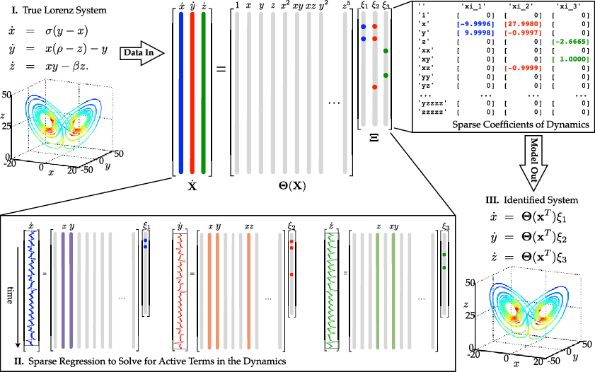
Illustration of the SINDy algorithm used on the Lorenz system. Credit to Brunton, Proctor, and Kutz.
A Brief Note about PySINDy
Before diving into the example code, it’s worth mentioning PySINDy, a Python package designed to streamline the implementation of SINDy algorithms. PySINDy aims to provide a broad framework for identifying governing equations from data, especially in systems where traditional methods may struggle due to complexity or sparsity. It’s designed to integrate well with NumPy and Scikit-learn.
We will NOT cover how to use PySINDy in this article. For those interested in exploring PySINDy on their own, you can check out the PySINDy documentation, browse the GitHub repository for code examples, or watch video tutorials to get started quickly. There’s also an introductory example that walks through how the algorithm works in practice.
The Lorenz System
The Lorenz system is a classic example of a chaotic dynamical system, originally developed by meteorologist Edward Lorenz in 1963 to model atmospheric convection. Its significance lies in its unpredictable, yet deterministic, nature, making it a popular subject in chaos theory. The system is governed by three ordinary differential equations (ODEs) involving three variables: \(x\), \(y\), and \(z\). Despite the simplicity of the equations, the Lorenz system exhibits highly complex, chaotic behavior, sensitive to initial conditions. Its chaotic nature makes it both fascinating and challenging to study, making it a perfect test case for SINDy. Check out an old post of mine about the Lorenz attractor!
Here are its governing equations:
The Lorenz system is particularly well-suited for testing SINDy because its underlying equations are parsimonious but generate rich, nonlinear dynamics. With just three simple equations, the system produces data that appears chaotic and difficult to model with traditional methods. However, SINDy’s strength lies in identifying the sparse structure behind such seemingly complex dynamics, making it a great tool for discovering the governing equations that might otherwise remain hidden.
In the next section, we’ll generate synthetic data by simulating the Lorenz system and use this data to apply the SINDy algorithm. Our goal is to see if SINDy can correctly predict the system’s underlying equations from the data, giving us a parsimonious model that explains the chaotic behavior. Let’s dive in and create some test data for the Lorenz system to start.
Start by installing all required Python packages:
pip install \derivative \matplotlib \numpy \scikit-learn \scipy
Note that aside from the typical Python packages used in data science (numpy, scipy, etc.) I also use methods from my own helpers module. You can find a copy of this module here.
import matplotlib.pyplot as pltimport numpy as npfrom derivative import dxdtfrom sklearn.linear_model import Lasso, ridge_regressionfrom sklearn.model_selection import train_test_splitfrom sklearn.preprocessing import StandardScaler# Import helper methods for plotting, etc. Find the code here:# https://gist.github.com/humatic/df255cda1731d5a1bb4bf9af0c744401from helpers import *
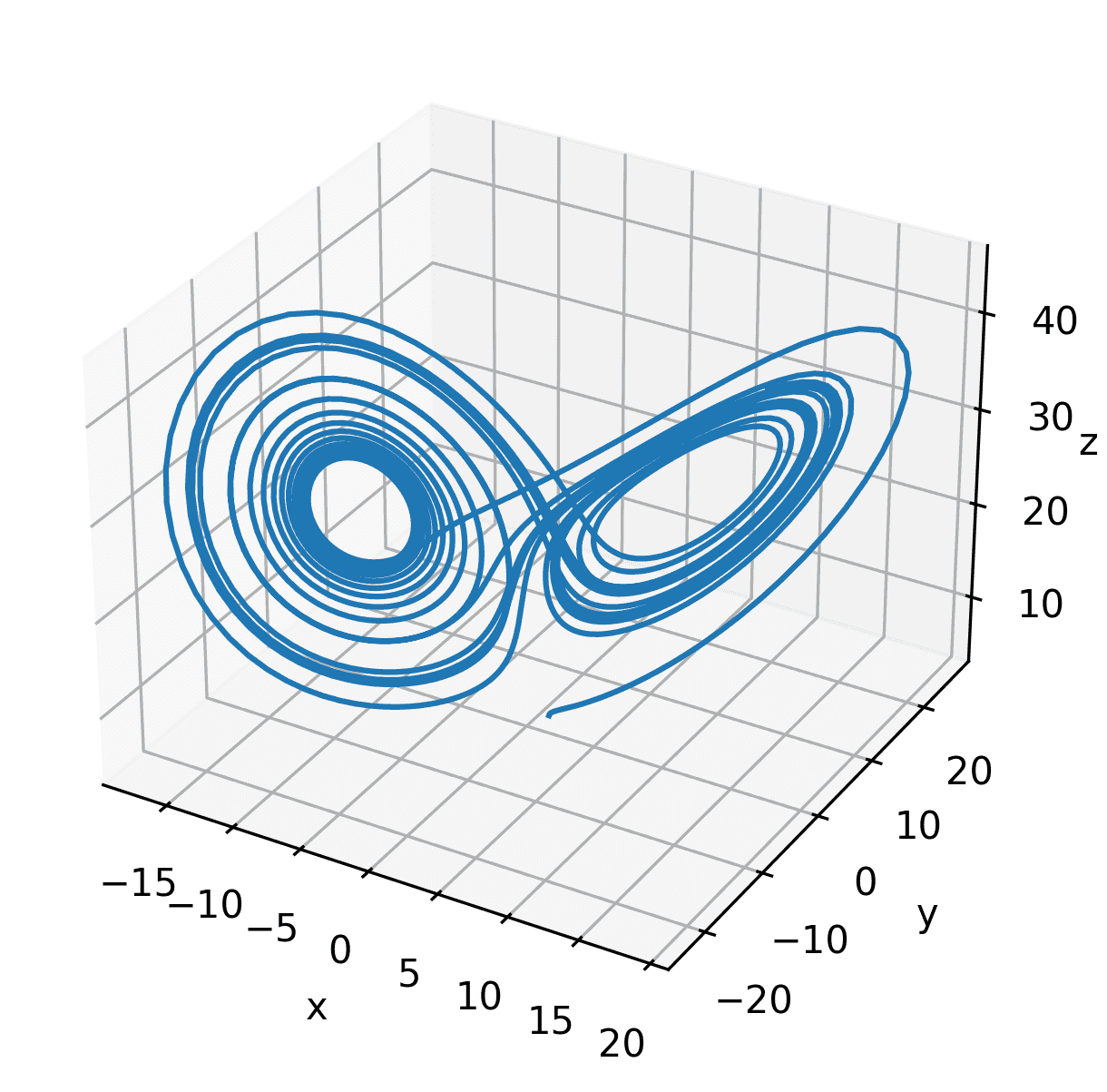
Our Lorenz data consists of three state variables in a matrix \(\mathbf{X}\) and their derivatives \(\mathbf{\dot{X}}\).
t_step = 0.01t_vec = np.arange(0, 100, t_step)X = integrate_lorenz(t_vec)dX = lorenz(t_vec, X)plot_lorenz_3d(X[:, :2000])
Example 1: State and Derivative Measurements
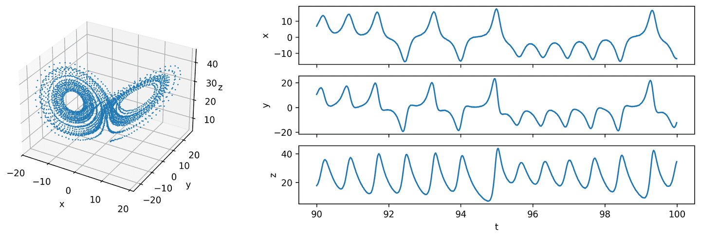
In our first example let’s assume that we possess measurement data for both the state and the derivative. We can synthesize the measurement data by adding a small amount of noise to the true state and derivative data (e.g. measurement error).
eta_1 = 0.01 # 1% noiseX_hat_1 = add_noise(X, eta_1)dX_hat_1 = add_noise(dX, eta_1)plot_lorenz(t_vec, X_hat_1)
Now let’s generate our feature library from the state measurements to produce \(\mathbb{\Theta}\). In the original SINDy paper they use polynomials — so that’s we’ll do too. More specifically, our feature library will consist of all polynomials derived from the state data of degree 5 or less.
theta_1, theta_cols = build_theta(X_hat_1, max_deg=5)
| 1 | x¹ | y¹ | z¹ | x² | x¹y¹ | y² | x¹z¹ | y¹z¹ | z² | … | x³z² | x²y¹z² | x¹y²z² | y³z² | x²z³ | x¹y¹z³ | y²z³ | x¹z⁴ | y¹z⁴ | z⁵ | |
|---|---|---|---|---|---|---|---|---|---|---|---|---|---|---|---|---|---|---|---|---|---|
| 0 | 1.0 | 1.56 | 0.18 | 4.83 | 2.42 | 0.28 | 0.03 | 7.52 | 0.88 | 23.34 | … | 8.80e+01 | 1.03e+01 | 1.21e+00 | 1.42e-01 | 2.73e+02 | 3.21e+01 | 3.76e+00 | 8.48e+02 | 9.95e+01 | 2.63e+03 |
| 1 | 1.0 | 1.53 | 0.53 | 4.84 | 2.33 | 0.80 | 0.28 | 7.38 | 2.55 | 23.41 | … | 8.31e+01 | 2.87e+01 | 9.94e+00 | 3.44e+00 | 2.64e+02 | 9.12e+01 | 3.16e+01 | 8.36e+02 | 2.89e+02 | 2.65e+03 |
| 2 | 1.0 | 1.38 | 0.83 | 4.46 | 1.91 | 1.14 | 0.69 | 6.15 | 3.69 | 19.86 | … | 5.23e+01 | 3.14e+01 | 1.88e+01 | 1.13e+01 | 1.69e+02 | 1.01e+02 | 6.08e+01 | 5.44e+02 | 3.27e+02 | 1.76e+03 |
| … | … | … | … | … | … | … | … | … | … | … | … | … | … | … | … | … | … | … | … | … | … |
| 9997 | 1.0 | -13.35 | -14.12 | 32.80 | 178.30 | 188.56 | 199.42 | -438.00 | -463.21 | 1075.95 | … | -2.56e+06 | -2.71e+06 | -2.87e+06 | -3.03e+06 | 6.29e+06 | 6.66e+06 | 7.04e+06 | -1.55e+07 | -1.63e+07 | 3.80e+07 |
| 9998 | 1.0 | -13.49 | -13.21 | 33.67 | 181.90 | 178.11 | 174.41 | -454.14 | -444.69 | 1133.85 | … | -2.78e+06 | -2.72e+06 | -2.67e+06 | -2.61e+06 | 6.94e+06 | 6.80e+06 | 6.66e+06 | -1.73e+07 | -1.70e+07 | 4.33e+07 |
| 9999 | 1.0 | -13.38 | -12.28 | 34.44 | 179.05 | 164.26 | 150.68 | -460.88 | -422.79 | 1186.28 | … | -2.84e+06 | -2.61e+06 | -2.39e+06 | -2.19e+06 | 7.32e+06 | 6.71e+06 | 6.16e+06 | -1.88e+07 | -1.73e+07 | 4.85e+07 |
10000 rows × 56 columns
What does the true Lorenz system look like when using the feature library? That’s where the sparse matrix \(\mathbb{\Xi}\) comes into play. We know that only certain entries in \(\mathbb{\Theta}\) are utilized in the true system, so \(\mathbb{\Xi}\) should be mostly zeros.
xi_true = get_xi_true(theta_cols)
| 1 | x¹ | y¹ | z¹ | x² | x¹y¹ | y² | x¹z¹ | y¹z¹ | z² | … | x³z² | x²y¹z² | x¹y²z² | y³z² | x²z³ | x¹y¹z³ | y²z³ | x¹z⁴ | y¹z⁴ | z⁵ | |
|---|---|---|---|---|---|---|---|---|---|---|---|---|---|---|---|---|---|---|---|---|---|
| 0 | 0.0 | -10.0 | 10.0 | 0.00 | 0.0 | 0.0 | 0.0 | 0.0 | 0.0 | 0.0 | … | 0.0 | 0.0 | 0.0 | 0.0 | 0.0 | 0.0 | 0.0 | 0.0 | 0.0 | 0.0 |
| 1 | 0.0 | 28.0 | -1.0 | 0.00 | 0.0 | 0.0 | 0.0 | -1.0 | 0.0 | 0.0 | … | 0.0 | 0.0 | 0.0 | 0.0 | 0.0 | 0.0 | 0.0 | 0.0 | 0.0 | 0.0 |
| 2 | 0.0 | 0.0 | 0.0 | -2.67 | 0.0 | 1.0 | 0.0 | 0.0 | 0.0 | 0.0 | … | 0.0 | 0.0 | 0.0 | 0.0 | 0.0 | 0.0 | 0.0 | 0.0 | 0.0 | 0.0 |
3 rows × 56 columns
Look carefully at the rows and columns in \(\mathbb{\Xi}\) and notice how the non-zero entries correspond to the parameters in the Lorenz system, namely \(\sigma=10\), \(\rho=28\), and \(\beta=8/3\). To make it even easier to interpret, let’s extract the non-zero coefficients and print them as a human-friendly system of equations.
print_system(xi_true, theta_cols)
Output:
dx = -10.000 x¹ + 10.000 y¹dy = 28.000 x¹ - 1.000 y¹ - 1.000 x¹z¹dz = -2.667 z¹ + 1.000 x¹y¹
Great, as expected! Now we can start digging into the primary focus of this article:
What if we don’t actually know about the underlying system of equations for the Lorenz model? Let’s imagine we just have the measurement data and nothing else. How to reveal those equations? We need a way to solve for \(\mathbb{\Xi}\).
Indeed there are many ways. In the next sections we’ll explore two methods: LASSO and the STLSQ algorithm.
LASSO Method
The first method is to use LASSO (least absolute shrinkage and selection operator). It is basically just a linear model trained with an \(L^1\) prior as regularizer. Here we’ll use the Scikit-learn implementation.
The most important hyperparameter for LASSO is probably \(\alpha\) — it controls the amount of \(L^1\) regularization. Higher \(\alpha\) will generally mean more sparsity in \(\mathbb{\Xi}\) and more parsimony in our final solution. So in our case, we want to see how high we can push \(\alpha\) without harming model accuracy.
def solve_with_lasso(X, y, scale=True, **kwargs):assert X.ndim == 2 and y.ndim == 2assert X.shape[0] == y.shape[0]# Optionally apply scaling to improve matrix conditioningif scale:scaler = StandardScaler(with_mean=False)X = scaler.fit_transform(X)# Do LASSO regressionkwargs.setdefault('alpha', 0.01)kwargs.setdefault('fit_intercept', False)kwargs.setdefault('precompute', True)kwargs.setdefault('max_iter', 20000)model = Lasso(**kwargs)model.fit(X, y)# Extract solved coef matrix and remove any scaling effectsxi = model.coef_if scale:xi = scaler.transform(xi)return xi
A couple things of note regarding our LASSO solver:
fit_interceptshould beFalsebecause our feature library already contains a column for constant coefficients (i.e. the first column)precomputeasTrueis better for much faster executionmax_iteroften needs to be higher than the default to achieve convergence
Also, you’ll notice that we scale theta with Scikit’s StandardScaler. This removes the variance of the features while leaving the mean intact.
- Removing the variance of the features is important because otherwise the solver may fail to converge (or at the very least spit out lots of
ConvergenceWarningwarnings). Note how we reverse the effect of the input scaling on our final solution by passing \(\mathbb{\Xi}\) through the same scaling procedure at the end. - Leaving the mean intact is convenient — although not strictly required — because otherwise each feature will have an additive component that will affect the distribution of sparse coefficients, making the solution slightly harder to interpret without additional steps.
Now let’s try it out on our measured data.
print('LASSO:\n')xi = solve_with_lasso(theta_1, dX_hat_1.T, alpha=0.01)coef_err = np.abs(xi - xi_true).sum()print_system(xi, theta_cols)print('err = %0.3f' % coef_err)
Output:
LASSO:dx = -9.358 x¹ + 9.683 y¹ - 0.020 x¹z¹ + 0.006 y¹z¹dy = 19.579 x¹ + 2.385 y¹ - 0.003 z¹ - 0.478 x¹z¹ - 0.127 y¹z¹ - 0.001 x¹y² - 0.008 x¹z²dz = -0.285 - 2.630 z¹ + 0.026 x² + 0.954 x¹y¹ + 0.014 y²err = 13.862
The result is “okay”. We can see the terms we were expecting, but their coefficients aren’t exactly right. Also, there are several unwanted terms. These not-quite-right results are likely due to biasing introduced into the solution by the \(L^1\) regularization term.
We can “debias” the solution by performing an extra round of regression, but without regularization. Simply filter out the near-zero coefficients from \(\mathbb{\Xi}\) (by choosing a threshold value), and then do a simple linear regression over the remaining coefficients only.
print('\nDebiased:\n')ind = np.abs(xi) >= 0.05xi = masked_linear_regression(theta_1, dX_hat_1.T, ind)coef_err = np.abs(xi - xi_true).sum()print_system(xi, theta_cols)print('err = %0.3f' % coef_err)
Output:
Debiased:dx = -9.992 x¹ + 9.993 y¹dy = 27.905 x¹ - 0.942 y¹ - 0.997 x¹z¹ - 0.002 y¹z¹dz = -0.017 - 2.666 z¹ + 1.000 x¹y¹err = 0.191
Much better results! There are only some minor discrepancies. And the error metric is really good!
So how can we pick an “ideal” value for \(\alpha\). What it boils down to is a hyperparameter search of some sort and there’s no single right way to do it. For larger models with lots of hyperparameters, you can use specialized libraries like Optuna to do the search. But for our small problem we’ll just plot out the so-called Pareto front.
def pareto_lasso(X, y, alpha_vec):# Split data for training and testingX_train, X_test, y_train, y_test = train_test_split(X, y, test_size=0.3, random_state=42)mse_vec = np.zeros(len(alpha_vec))for i, alpha in enumerate(alpha_vec):# Solve for xi with LASSOxi = solve_with_lasso(X_train, y_train, alpha=alpha, precompute=True)ind = np.abs(xi) >= 0.05xi = masked_linear_regression(X_train, y_train, ind)# Compute MSE of test prediction produced by xiy_pred = X_test @ xi.Tmse_vec[i] = ((y_test - y_pred)**2).mean()return mse_vecalpha_vec = np.logspace(-3, 0, 50)mse_vec = pareto_lasso(theta_1, dX_hat_1.T, alpha_vec)plot_pareto_lasso(mse_vec, alpha_vec, log=True)
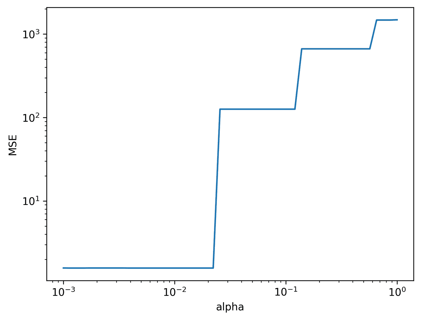
Remember: we want to push \(\alpha\) as high as possible without introducing unnecessary error. Judging by the curve, we can see that \(\alpha\approx0.01\) may be the best choice.
STLSQ Method
Now let’s replace LASSO with a novel method introduced by the authors of the original SINDy paper — the Sequentially Thresholded Least Squares (STLSQ) algorithm. At its core it’s very simple: all it does is alternate between finding a least-squares solution for the coefficient matrix and then “zeroing out” any coefficients smaller than a given threshold. Rinse and repeat several times and eventually the algorithm converges to a sparse solution \(\mathbb{\Xi}\). Then we can debias the coefficients (same as before) and we have our solution!
Here’s a pure Python implementation of the algorithm, complete with scaling and debiasing (see notes in previous section). Note that in this implementation, \(\alpha\) is used for a ridge regression which utilizes an \(L^2\) regularizer rather than \(L^1\) regularizer. This is how the PySINDy authors have done it and it works fine. I suspect that one could swap out the regression method for another type if desired. The important bit is that the regression method includes a mechanism to penalize coefficients that serve little purpose.
def solve_with_stlsq(X,y,max_iter=20,threshold=0.01,alpha=0.1,scale=True,debias=True,):assert X.ndim == 2 and y.ndim == 2assert X.shape[0] == y.shape[0]assert max_iter > 0assert threshold >= 0assert alpha >= 0# Data dimensionsn_samp, n_feat = X.shapen_targ = y.shape[1]# Optionally apply scaling to improve matrix conditioningif scale:scaler = StandardScaler(with_mean=False)X = scaler.fit_transform(X)# Indexing matrix initialized to all True, but will eventually# become sparse as the solution convergesind = np.ones((n_targ, n_feat), dtype=bool)prev_ind = Nonefor k in range(max_iter):# Find best coefficients for each targetcoef = np.zeros((n_targ, n_feat))for i in range(n_targ):# At least one non-zero target requiredif np.count_nonzero(ind[i]) == 0:continue# Ridge regressioncoef[i, ind[i]] = ridge_regression(X[:, ind[i]], y[:, i], alpha)# Reverse effects of optional scalingif scale:coef = scaler.transform(coef)# Apply thresholdingind = np.abs(coef) >= thresholdcoef[~ind] = 0# Check if the coefficient mask has changed after thresholdingif prev_ind is not None and (ind == prev_ind).all():breakprev_ind = ind.copy()else:print(f'STLSQ did not converge after {max_iter} iterations')# Optionally debias the coefficients by regressing over the sparse# indices without any regularization (i.e. vanilla linear regression)if debias:coef = masked_linear_regression(X, y, ind)if scale:coef = scaler.transform(coef)return coef, ind
Applying it to our measurement data and we get even better results than with LASSO!
xi, xi_ind = solve_with_stlsq(theta_1, dX_hat_1.T, alpha=0.1, threshold=0.1)coef_err = np.abs(xi - xi_true).sum()print_system(xi, theta_cols)print('err = %0.3f' % coef_err)
Output:
dx = -9.992 x¹ + 9.993 y¹dy = 27.974 x¹ - 0.992 y¹ - 0.999 x¹z¹dz = -2.666 z¹ + 1.000 x¹y¹err = 0.051
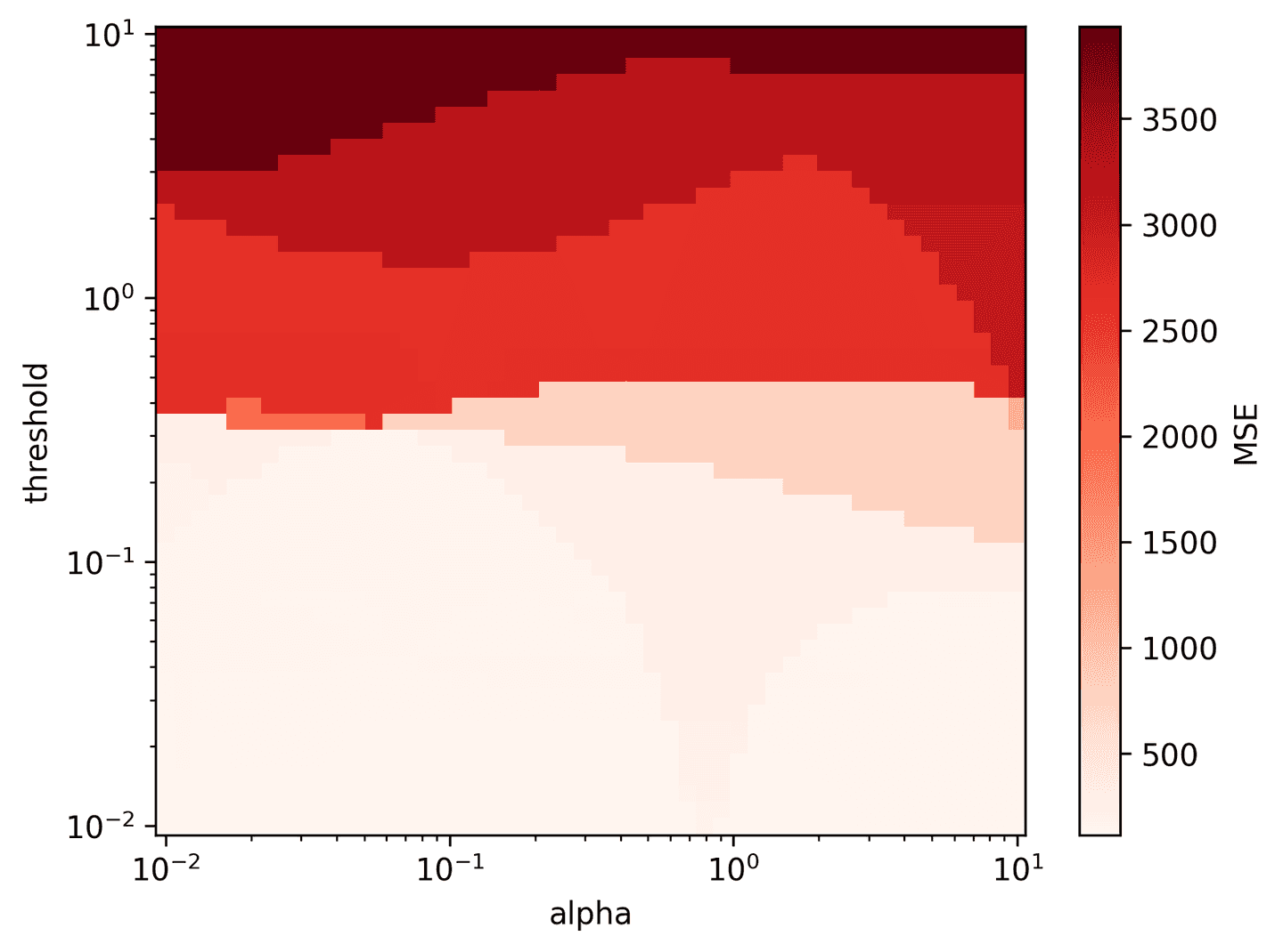
The STLSQ has two main hyperparameters of interest: alpha and threshold. Let’s search the 2D hyperparameter space and create a heat map of the mean squared error.
def pareto_stlsq(X, y, alpha_vec, threshold_vec):# Split data for training and testingX_train, X_test, y_train, y_test = train_test_split(X, y, test_size=0.3, random_state=42)mse_mat = np.zeros((len(alpha_vec), len(threshold_vec)))total = mse_mat.sizeprog = 0for i, alpha in enumerate(alpha_vec):for j, threshold in enumerate(threshold_vec):# Solve for xi with STLSQxi, xi_ind = solve_with_stlsq(X_train, y_train, alpha=alpha, threshold=threshold)# Compute MSE of test prediction produced by xiy_pred = X_test @ xi.Tmse_mat[i, j] = ((y_test - y_pred)**2).mean()# Progress updateprog += 1if (prog % 500 == 0) or prog == total:print(f'{prog}/{total}')return mse_matalpha_vec = np.logspace(-2, 1, 50)threshold_vec = np.logspace(-2, 1, 50)mse_mat = pareto_stlsq(theta_1, dX_hat_1.T, alpha_vec, threshold_vec)plot_pareto_stlsq(mse_mat, alpha_vec, threshold_vec, log=True)
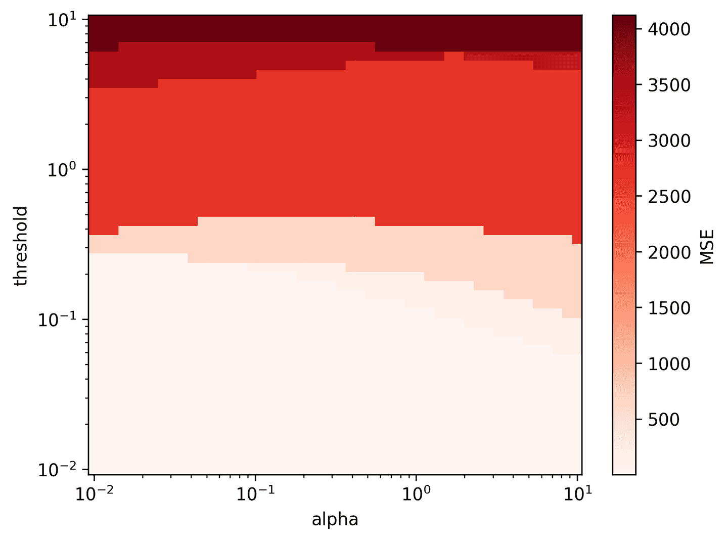
It looks like a wide range of parameters result in low MSE. alpha=0.1 and threshold=0.1 are simple choices that appear to work well.
Example 2: Noisy State Measurements Only
For our next example, let’s bump up the difficulty a bit by:
- Only utilizing state measurements (so no access to derivative measurements)
- Adding higher noise to the state (10% error rather than 1%)
Like so:
eta_2 = 0.1 # 10% noiseX_hat_2 = add_noise(X, eta_2)theta_2, theta_cols = build_theta(X_hat_2, max_deg=5)plot_lorenz(t_vec, X_hat_2)
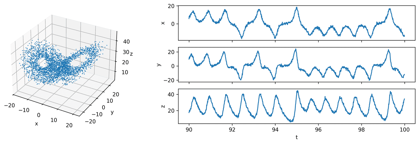
The biggest hurdle to clear is the lack of data for the left-hand side of our regression problem. How to find the optimum coefficient matrix that results in accurate derivatives if we don’t know what the derivatives should be?
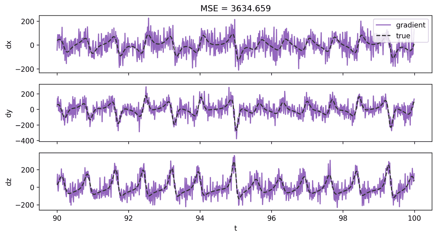
We have data for \(\mathbf{X}\), so it should be possible to approximate \(\mathbf{\dot X}\) computationally. A simple approach would be to compute finite differences using methods like numpy.diff or numpy.gradient. But when there’s noise involved, these methods will likely just amplify the error. For example, here’s what the state derivative looks like when estimating it with numpy.gradient. Very noisy!
dX_grad_2 = np.gradient(X_hat_2, t_step, axis=1)plot_lorenz_deriv_with_est(t_vec, dX, dX_grad_2, 'gradient')
Measurement Filter
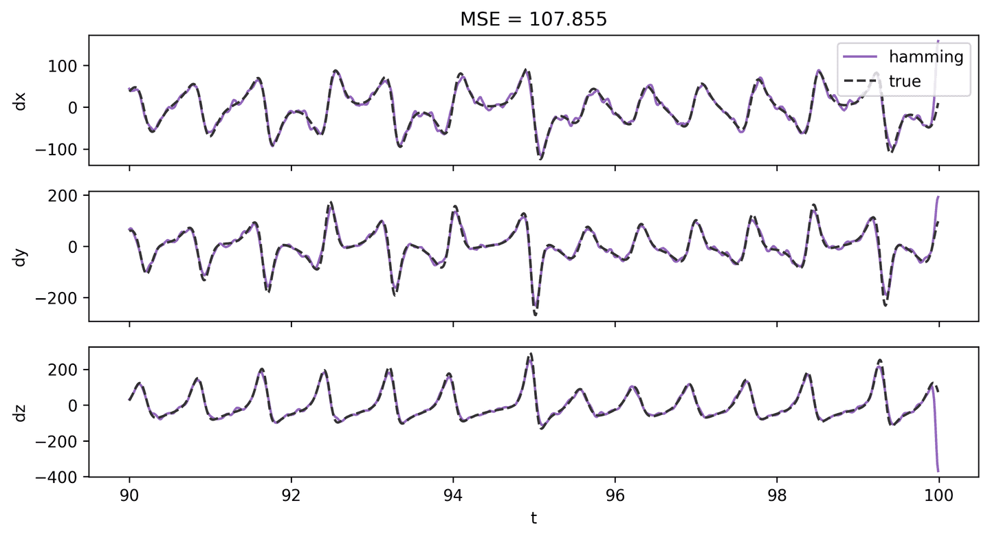
A better approach is to try and reduce the noise in the state using a filter of some sort prior to computing the derivative. Here’s an example of a derivative estimation after applying a Hamming filter to the state measurements.
The result is clearly better, both visually and in terms of MSE!
def hamming_filter(X, m=15):ham = np.hamming(m)ham /= ham.sum()X_ham = np.zeros_like(X)for i in range(len(X)):X_ham[i] = np.convolve(X[i], ham, mode='same')return X_hamX_ham_2 = hamming_filter(X_hat_2)dX_ham_2 = np.gradient(X_ham_2, t_step, axis=1)plot_lorenz_deriv_with_est(t_vec, dX, dX_ham_2, 'hamming')
Derivative Estimation
But we can do even better.
There are more advanced methods available made specifically for derivative estimation. Check out the derivative Python package, part of the PySINDy project. It offers many great methods, including finite differences, Kalman derivative, the total variation regularized derivative (TVRD), and others.
The authors of the original SINDy paper used the TVRD method. But in my experience I found the TVRD implementation from derivative to be super costly computationally.
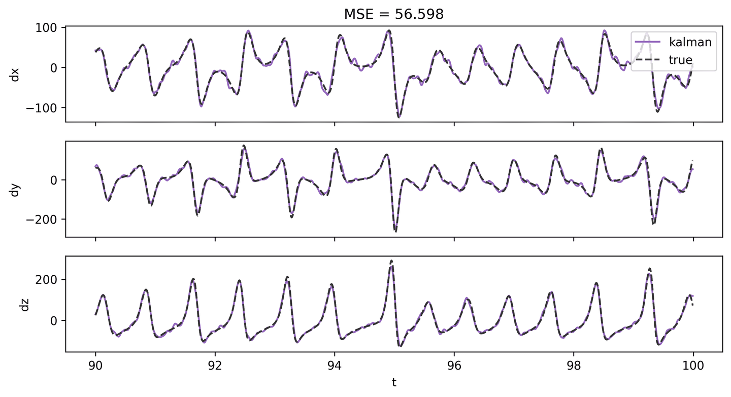
Instead, I suggest trying the Kalman. It gives great results with reasonable performance. We’ll use this derivative for subsequent steps.
dX_kal_2 = dxdt(X_hat_2, t_vec, kind='kalman', alpha=0.00005)plot_lorenz_deriv_with_est(t_vec, dX, dX_kal_2, 'kalman')
Apply the STLSQ
Almost there! Let’s just do a quick search of the STLSQ hyperparameter space for nice parameter values. Looks like alpha=0.1 and threshold=0.2 may work best.
alpha_vec = np.logspace(-2, 1, 50)threshold_vec = np.logspace(-2, 1, 50)mse_mat = pareto_stlsq(theta_2, dX_kal_2.T, alpha_vec, threshold_vec)plot_pareto_stlsq(mse_mat, alpha_vec, threshold_vec, log=True)
Finally let’s apply the STLSQ algorithm to solve for the Lorenz equations.
xi, xi_ind = solve_with_stlsq(theta_2, dX_kal_2.T, alpha=0.1, threshold=0.2)coef_err = np.abs(xi - xi_true).sum()print_system(xi, theta_cols)print('err = %0.3f' % coef_err)
Output:
dx = 0.223 - 9.030 x¹ + 9.108 y¹dy = -0.505 + 23.004 x¹ + 0.304 y¹ - 0.877 x¹z¹dz = -0.387 - 2.531 z¹ + 0.956 x¹y¹err = 9.580
As you can see, we arrived at a set of equations that mostly line up with the true, expected Lorenz system. And the coefficient error is reasonable. Given the extra noise and the lack of derivative measurements I’d say we did pretty good!
LASSO vs. STLSQ
This article presents both the LASSO and the STLSQ algorithm as methods for identifying unknown systems of equations with SINDy. Both seemed to work well — at least for the mocked up Lorenz examples above. Before closing I just want to touch on some of the key differences between the two methods.
- Quality: In low-noise contexts, both the LASSO and the STLSQ perform well. However, in high-noise contexts, the STLSQ generally yields much better results, at least in my experience.
- Flexibility: I’ve found the STLSQ to be highly versatile. Not only does it have more hyperparameters to tweak, but you can even potentially swap out the convergence criteria and/or the underlying regression routines. LASSO on the other hand — despite being very powerful in its own right — is more of a one-trick pony when it comes to SINDy.
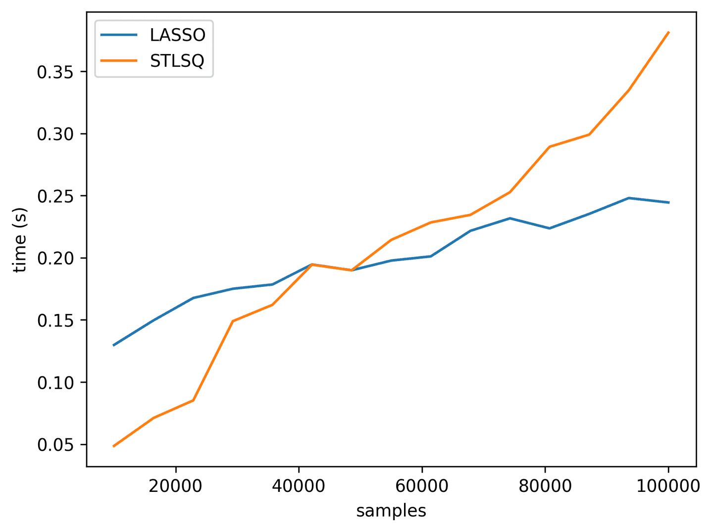
- Performance: Speed-wise, both methods are roughly comparable, although the LASSO may scale slightly better (see graph below). Don’t forget to use
precompute=Truefor LASSO! As memory requirements increase (e.g. larger data matrices), both of these methods will eventually hit a ceiling because of the in-memory nature of the regression methods under the hood. If that happens you’ll likely need to find a way to reduce the dimensionality of the data or to split it into smaller batches.
def _lasso(*args):xi = solve_with_lasso(*args)ind = np.abs(xi) >= 0.05masked_linear_regression(*args, ind)lasso_perf = []stlsq_perf = []for t_stop in np.linspace(100, 1000, 15):print(int(t_stop))avg, n_samp, n_feat = test_perf(_lasso, t_stop=t_stop)lasso_perf.append((n_samp, avg))avg, n_samp, n_feat = test_perf(solve_with_stlsq, t_stop=t_stop)stlsq_perf.append((n_samp, avg))plt.plot(*zip(*lasso_perf), label='LASSO')plt.plot(*zip(*stlsq_perf), label='STLSQ')plt.xlabel('samples')plt.ylabel('time (s)')plt.legend()
Summary
This guide explores how SINDy (Sparse Identification of Nonlinear Dynamics) can help us uncover the rules governing complex systems, using only data instead of traditional trial and error. SINDy simplifies a system’s behavior by identifying just the most essential factors, giving us a clear, interpretable model. We apply this approach to the chaotic Lorenz system — a well-known example in weather modeling and chaos theory — to see if SINDy can reveal its core equations. Along the way, we compare two methods, LASSO and STLSQ, showing how SINDy manages both noisy data and missing information to make reliable predictions about complex systems.
Resources
- Brunton, S. L., Proctor, J. L., & Kutz, J. N. (2016). Discovering governing equations from data by sparse identification of nonlinear dynamical systems. Proceedings of the national academy of sciences, 113(15), 3932-3937.
- Brunton, S. L., Proctor, J. L., & Kutz, J. N. (2016). Sparse identification of nonlinear dynamics with control (SINDYc). IFAC-PapersOnLine, 49(18), 710-715.
- Kaiser, E., Kutz, J. N., & Brunton, S. L. (2018). Sparse identification of nonlinear dynamics for model predictive control in the low-data limit. Proceedings of the Royal Society A, 474(2219), 20180335.
- de Silva, B. M., Champion, K., Quade, M., Loiseau, J. C., Kutz, J. N., & Brunton, S. L. (2020). Pysindy: a python package for the sparse identification of nonlinear dynamics from data. arXiv preprint arXiv:2004.08424.
- Champion, K., Zheng, P., Aravkin, A. Y., Brunton, S. L., & Kutz, J. N. (2020). A unified sparse optimization framework to learn parsimonious physics-informed models from data. IEEE Access, 8, 169259-169271.
- Kutz, J. N., & Brunton, S. L. (2022). Parsimony as the ultimate regularizer for physics-informed machine learning. Nonlinear Dynamics, 107(3), 1801-1817.
- Kaptanoglu, A. A., de Silva, B. M., Fasel, U., Kaheman, K., Goldschmidt, A. J., Callaham, J. L., … & Brunton, S. L. (2021). PySINDy: A comprehensive Python package for robust sparse system identification. arXiv preprint arXiv:2111.08481.
- Delahunt, C. B., & Kutz, J. N. (2022). A toolkit for data-driven discovery of governing equations in high-noise regimes. IEEE Access, 10, 31210-31234.
- Wikipedia contributors. (2024, September 17). Lorenz system. In Wikipedia, The Free Encyclopedia. Retrieved 18:18, October 16, 2024, from https://en.wikipedia.org/w/index.php?title=Lorenz_system&oldid=1246222439
- Wikipedia contributors. (2024, September 21). Ridge regression. In Wikipedia, The Free Encyclopedia. Retrieved 17:59, October 16, 2024, from https://en.wikipedia.org/w/index.php?title=Ridge_regression&oldid=1246894940
GET IN TOUCH
Have a project in mind?
Reach out directly to hello@humaticlabs.com or use the contact form.