Optimal Singular Value Hard Threshold

Rank-reduction is a very common task in many SVD-based methods and algorithms. It is the technique by which a high-dimensional, noisy data set can be reduced to a low-dimensional, clean(er) data set. Under ideal circumstances, an “in-the-loop” human expert will perform the rank-reduction according to their own judgment. Unfortunately, expert knowledge is often unavailable for automated methods and algorithms. This post demonstrates a principled approach for performing the reduction auto-magically — without any need for expert, “in-the-loop” knowledge!

Recall that the SVD of an m-by-n data matrix \(D\) looks like this:

One of the first steps after SVD-ing your data matrix is to take a quick look that the singular values in \(\Sigma\). Usually, the “look and feel” of the singular values will tell you something about the ideal dimensionality, or rank, of the data. Once you decide on a new rank, r, you can truncate the \(U\Sigma V^*\) matrices accordingly to simplify the system.

There are many techniques out there that attempt to automate the determination of r. One such technique is the Optimal Singular Value Hard Threshold (optimal SVHT) developed by Gavish and Donoho (2014). Here I’ve extracted the key ideas from their article and recast them in a Python context.

The Basics

Let’s start off by building a test data matrix that we know contains some structure and some noise. Arbitrarily, we choose the x-axis to represent a single spatial dimension and the y-axis to represent time. The axes could represent anything though — the SVD will handle any 2D matrix.

import numpy as np
import matplotlib.pyplot as plt
from numpy import dot, diag, exp, real, sin, cosh, tanh
from scipy.linalg import svd, svdvals

# define time and space domains
x = np.linspace(-10, 10, 100)
t = np.linspace(0, 20, 200)
Xm,Tm = np.meshgrid(x, t)

# create data
D = 5 * (1/cosh(Xm/2)) * tanh(Xm/2) * exp((1.5j)*Tm) # primary mode
D += 0.5 * sin(2 * Xm) * exp(2j * Tm)                # secondary mode
D += 0.5 * np.random.randn(*Xm.shape)                # noise

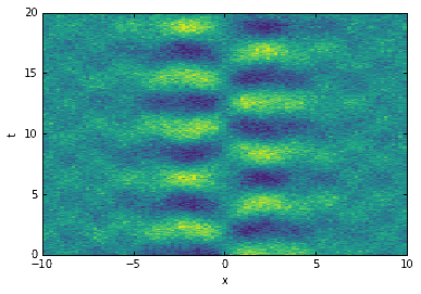
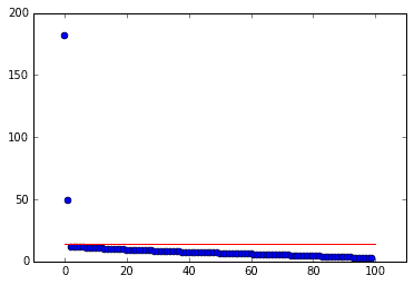
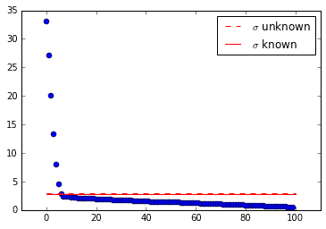
If you study the code, you’ll notice that the data contains two modes and a small amount of normally distributed noise, with \(\sigma=1/2\). When plotting the singular values of \(D\), one would expect to see two large, well-separated singular values with the remainder being much smaller and tapering off towards zero (as we shall see, that is exactly what happens). The rank should be \(r=2\).

The optimal SVHT, \(\tau_*\), tells us approximately where to truncate the singular values so that only “important” modes remain. The calculation of \(\tau_*\) falls into one of two general scenarios: where the noise level \(\sigma\) is known or unknown. I would assume that \(\sigma\) is unknown in most cases of interest, so we’ll start with that.

For \(\sigma\) unknown, the optimal SVHT can be estimated with

where \(\beta=m/n\) (with \(m\le n\)), \(y_{\textit{med}}\) is the median singular value of the data matrix \(D\), and \(\omega(\beta)\) can be approximated with

Note that an exact computation of \(\omega\) is possible (but not included here). It requires that you numerically compute \(\mu_\beta\), the median of the Marchenko-Pastur distribution. Gavish and Donoho provide a MATLAB source code supplement that demonstrates how to do this. Also look at this github project for an example written in Python. Once you have \(\mu_\beta\), then the exact \(\omega\) is given by

The quantity \(\lambda_*(\beta)\) shall be explained shortly. For now, let’s SVD the data matrix and compute \(\tau_*\).

def omega_approx(beta):
    """Return an approximate omega value for given beta. Equation (5) from Gavish 2014."""
    return 0.56 * beta**3 - 0.95 * beta**2 + 1.82 * beta + 1.43

# do SVD and find tau star hat
U,sv,Vh = svd(D, False)
beta = min(D.shape) / max(D.shape)
tau = np.median(sv) * omega_approx(beta)

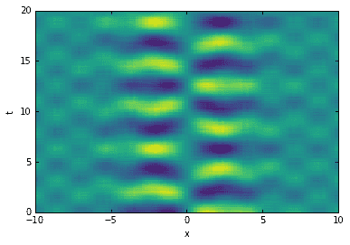
In the plot of singular values above, the red line indicates \(\tau_*\). Notice how it conveniently separates the true modes from the garbage. Now that we have the optimal SVHT, we can truncate the SVD and reconstruct the data. The new data matrix will be the same as before, but de-noised!

# reconstruct data (de-noised)
sv2 = sv.copy()
sv2[sv < tau] = 0
D2 = dot(dot(U, diag(sv2)), Vh)

When \(\sigma\) is known, the formulation is slightly different:

It is important to note that \(n\) is assumed to be the larger of the two dimensions. The quantity \(\lambda_*(\beta)\) is given by

The following code calculates \(\tau_*\) for \(D\) with \(\sigma=1/2\).

def lambda_star(beta):
    """Return lambda star for given beta. Equation (11) from Gavish 2014."""
    return np.sqrt(2 * (beta + 1) + (8 * beta) / 
                   (beta + 1 + np.sqrt(beta**2 + 14 * beta + 1)))

# find tau star
tau = lambda_star(beta) * np.sqrt(max(D.shape)) * 0.5

Convenience method

I wrote the following method to conveniently handle the computation of \(\tau_*\) for most use cases. Just copy and paste it, including the imports from before.

def svht(X, sigma=None, sv=None):
    """Return the optimal singular value hard threshold (SVHT) value.
    `X` is any m-by-n matrix. `sigma` is the standard deviation of the 
    noise, if known. Optionally supply the vector of singular values `sv`
    for the matrix (only necessary when `sigma` is unknown). If `sigma`
    is unknown and `sv` is not supplied, then the method automatically
    computes the singular values."""
    
    try:
        m,n = sorted(X.shape) # ensures m <= n
    except:
        raise ValueError('invalid input matrix')
    beta = m / n # ratio between 0 and 1
    if sigma is None: # sigma unknown
        if sv is None:
            sv = svdvals(X)
        sv = np.squeeze(sv)
        if sv.ndim != 1:
            raise ValueError('vector of singular values must be 1-dimensional')
        return np.median(sv) * omega_approx(beta)
    else: # sigma known
        return lambda_star(beta) * np.sqrt(n) * sigma

# find tau star hat when sigma is unknown
tau = svht(D, sv=sv)

# find tau star when sigma is known
tau = svht(D, sigma=0.5)

Completely Random Matrix

The first example matrix contained clear structure. Let’s test the strategy for a completely random matrix. We see that the optimal SVHT tells us to truncate everything!

# create matrix of random data
D = np.random.randn(100, 100)

# do SVD and find tau stars
U,sv,Vh = svd(D, False)
tau1 = svht(D, sv=sv) # sigma unknown
tau2 = svht(D, sigma=1) # sigma known

Translational Invariance

It happens sometimes that a data set is low-dimensional, but its SVD suggests high-dimensionality. Translational invariance is one such case. Let’s see how the optimal SVHT holds up to weird data like this.

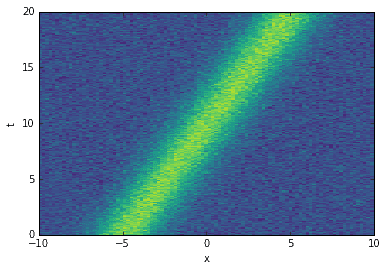
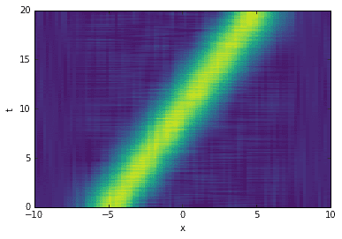
The following data matrix contains a single mode (a Gaussian) moving diagonally through space and time. Sadly, the SVD is not able to isolate the single mode. It identifies many modes instead.

The cool thing is that (at least in this case) the optimal SVHT is still useful! The truncation thresholds shown in the singular value plot below are intuitive.

# create data with a single mode traveling both spatially and in time
D = exp(-np.power((Xm-(Tm/2)+5)/2, 2))
D += 0.1 * np.random.randn(*Xm.shape) # noise

# do SVD and find tau stars
U,sv,Vh = svd(D, False)
tau1 = svht(D, sv=sv) # sigma unknown
tau2 = svht(D, sigma=0.1) # sigma known

Truncate the SVD and reconstruct the data with fewer dimensions to produce a cleaner image. Even though the SVD fails to pick up the single mode, the SVHT still recommends a sensible rank for row-reduction.

# reconstruct data (de-noised)
sv2 = sv.copy()
sv2[sv < tau1] = 0
D2 = dot(dot(U, diag(sv2)), Vh)

References

1. Gavish, Matan, and David L. Donoho. “The optimal hard threshold for singular values is.” IEEE Transactions on Information Theory 60.8 (2014): 5040-5053.
2. Gavish, Matan, and David L. Donoho. Code supplement to “The optimal hard threshold for singular values is.” [Online]. Available: http://purl.stanford.edu/vg705qn9070
3. Wikipedia contributors. “Marchenko–Pastur distribution.” Wikipedia, The Free Encyclopedia. Wikipedia, The Free Encyclopedia, 29 May. 2016. Web. 31 Jul. 2016.