Multi-resolution DMD

Previously, I investigated the dynamic mode decomposition (DMD) and the sparsity-promoting dynamic mode decomposition (spDMD). This time I am posting about the multi-resolution DMD — another extension to the DMD, recently developed by Kutz, Fu, and Brunton.

The mrDMD is a very powerful and general method for extracting dynamic structures from time-series data. Its primary strength stems from its ability to identify features at varying time scales. It does so by recursively parsing through the data set, performing the DMD on different subsamples. The resulting output then provides a means to better analyze the underlying dynamics of the data at different scales and to even perform fine-grained predictions.

We start by constructing a toy example containing features at multiple time scales, including one-time events. The normal DMD fails to capture some of the features because it is poor at handling “weird” data containing transient phenomena. Then, we summarize the mrDMD procedure and test it on the data. The mrDMD yields a very accurate reconstruction of the data.

Multi-resolution Data

import numpy as np
import matplotlib.pyplot as plt
from numpy import dot, multiply, diag, power
from numpy import pi, exp, sin, cos
from numpy.linalg import inv, eig, pinv, solve
from scipy.linalg import svd, svdvals
from math import floor, ceil # python 3.x

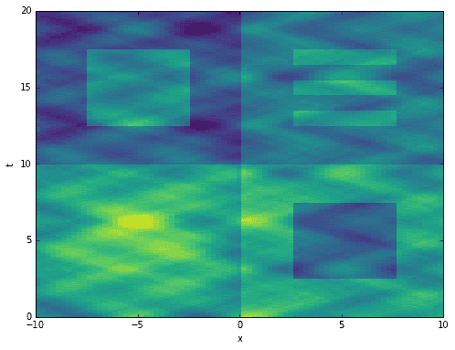
The code below generates toy data with a single spatial dimension and a time dimension. The data can be thought of as 80 locations or signals (the x-axis) being sampled 1600 times at a constant rate in time (the t-axis). It contains many features at varying time scales. Some are oscillating sines and cosines. Others are unpredictable, one-time events. The data is entirely arbitrary and has no real-world relevance.

# define time and space domains
x = np.linspace(-10, 10, 80)
t = np.linspace(0, 20, 1600)
Xm,Tm = np.meshgrid(x, t)

# create data
D = exp(-power(Xm/2, 2)) * exp(0.8j * Tm)
D += sin(0.9 * Xm) * exp(1j * Tm)
D += cos(1.1 * Xm) * exp(2j * Tm)
D += 0.6 * sin(1.2 * Xm) * exp(3j * Tm)
D += 0.6 * cos(1.3 * Xm) * exp(4j * Tm)
D += 0.2 * sin(2.0 * Xm) * exp(6j * Tm)
D += 0.2 * cos(2.1 * Xm) * exp(8j * Tm)
D += 0.1 * sin(5.7 * Xm) * exp(10j * Tm)
D += 0.1 * cos(5.9 * Xm) * exp(12j * Tm)
D += 0.1 * np.random.randn(*Xm.shape)
D += 0.03 * np.random.randn(*Xm.shape)
D += 5 * exp(-power((Xm+5)/5, 2)) * exp(-power((Tm-5)/5, 2))
D[:800,40:] += 2
D[200:600,50:70] -= 3
D[800:,:40] -= 2
D[1000:1400,10:30] += 3
D[1000:1080,50:70] += 2
D[1160:1240,50:70] += 2
D[1320:1400,50:70] += 2
D = D.T

# extract input-output matrices
X = D[:,:-1]
Y = D[:,1:]

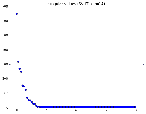
It is always important to first take a quick look at the data’s singular values. Here we use the optimal SVHT to cut away noise and determine the optimal rank for rank reduction (code copied and simplified from previous post). The red line in the singular value plot is the optimal SVHT. Anything above the line, we keep; anything below can be discarded.

def svht(X, sv=None):
    # svht for sigma unknown
    m,n = sorted(X.shape) # ensures m <= n
    beta = m / n # ratio between 0 and 1
    if sv is None:
        sv = svdvals(X)
    sv = np.squeeze(sv)
    omega_approx = 0.56 * beta**3 - 0.95 * beta**2 + 1.82 * beta + 1.43
    return np.median(sv) * omega_approx

# determine rank-reduction
sv = svdvals(X)
tau = svht(X, sv=sv)
r = sum(sv > tau)

Here I’m declaring the dmd method originally derived in my post on the DMD in Python.

def dmd(X, Y, truncate=None):
    if truncate == 0:
        # return empty vectors
        mu = np.array([], dtype='complex')
        Phi = np.zeros([X.shape[0], 0], dtype='complex')
    else:
        U2,Sig2,Vh2 = svd(X, False) # SVD of input matrix
        r = len(Sig2) if truncate is None else truncate # rank truncation
        U = U2[:,:r]
        Sig = diag(Sig2)[:r,:r]
        V = Vh2.conj().T[:,:r]
        Atil = dot(dot(dot(U.conj().T, Y), V), inv(Sig)) # build A tilde
        mu,W = eig(Atil)
        Phi = dot(dot(dot(Y, V), inv(Sig)), W) # build DMD modes
    return mu, Phi

Now let’s compute the DMD. After that, compute the time evolution resulting from initial row of data. Notice that when we plot the reconstruction, it completely fails to approximate the original data! Clearly some features are captured, but transient time events are mostly missing.

# do dmd
mu,Phi = dmd(X, Y, r)

# compute time evolution
b = dot(pinv(Phi), X[:,0])
Vand = np.vander(mu, len(t), True)
Psi = (Vand.T * b).T

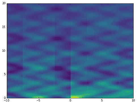
This is one of the weaknesses of the DMD. My previous post on the DMD shows this idea more concisely. Fortunately, the mrDMD sidesteps this issue completely.

mrDMD Concepts and Code

Now for a tiny bit of theory. The first main concept to understand is that each DMD mode has a relative frequency and/ or decay rate determined by its eigenvalue \(\mu\). One might think of it as the mode’s “speed” — a fast mode oscillates/ grows/ decays rapidly, while a slow mode takes its time. If we recall the form of the equations for the time dynamics of a mode, it becomes clear that a mode’s speed should be proportional to \(\lvert\ln(\mu)\rvert\). The exact speed depends entirely on the units of time and how the data is being sampled.

So, a mode can be considered “slow” if it has a relatively low frequency or slow growth/ decay rate. This just means that the mode changes somewhat slowly as the system evolves in time.

Consider the following plot of logs of the eigenvalues computed earlier. In particular, notice that a dotted circle of arbitrary radius is also plotted to illustrate a possible distinction between “slow” and “fast” modes. We could potentially decide that all eigenvalues within that circle correspond to slow modes while the rest correspond to fast modes.

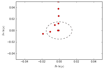
The reason I mention eigenvalues and mode “speed” is that the mrDMD recursively extracts the “slow” modes at each time scale that it evaluates. What constitutes “slow” or “fast” depends entirely on the eigenvalue in question and what time scale it belongs to.

The general mrDMD algorithm is as follows:

1. Compute DMD for available data.
2. Determine fast and slow modes.
3. Find the best DMD approximation to the available data constructed from the slow modes only.
4. Subtract off the slow-mode approximation from the available data.
5. Split the available data in half.
6. Repeat the procedure for the first half of data (including this step).
7. Repeat the procedure for the second half of data (including this step).

These are the basic steps. A few notes:

• The procedure is recursive.
• For better execution time, we subsample the data at each level of the recursion. This entails recasting the data such that its new size is the minimum necessary to capture any slow modes.
• At each level we can perform rank-reduction using the optimal SVHT.
• Step 3 requires us to compute the “best DMD approximation”. We use the optimal \(b\) computation for this step (borrowed from the spDMD). See my post on the spDMD for more explanation.
• Once we know the optimal \(b\) vector, we can construct a slow-mode approximation to the data. The approximation is then subtracted from the data available at that current level to produce a new data set for the subsequent level.

Below is my annotated version of the mrDMD in Python.

def mrdmd(D, level=0, bin_num=0, offset=0, max_levels=7, max_cycles=2, do_svht=True):
    """Compute the multi-resolution DMD on the dataset `D`, returning a list of nodes
    in the hierarchy. Each node represents a particular "time bin" (window in time) at
    a particular "level" of the recursion (time scale). The node is an object consisting
    of the various data structures generated by the DMD at its corresponding level and
    time bin. The `level`, `bin_num`, and `offset` parameters are for record keeping 
    during the recursion and should not be modified unless you know what you are doing.
    The `max_levels` parameter controls the maximum number of levels. The `max_cycles`
    parameter controls the maximum number of mode oscillations in any given time scale 
    that qualify as "slow". The `do_svht` parameter indicates whether or not to perform
    optimal singular value hard thresholding."""

    # 4 times nyquist limit to capture cycles
    nyq = 8 * max_cycles

    # time bin size
    bin_size = D.shape[1]
    if bin_size < nyq:
        return []

    # extract subsamples 
    step = floor(bin_size / nyq) # max step size to capture cycles
    _D = D[:,::step]
    X = _D[:,:-1]
    Y = _D[:,1:]

    # determine rank-reduction
    if do_svht:
        _sv = svdvals(_D)
        tau = svht(_D, sv=_sv)
        r = sum(_sv > tau)
    else:
        r = min(X.shape)

    # compute dmd
    mu,Phi = dmd(X, Y, r)

    # frequency cutoff (oscillations per timestep)
    rho = max_cycles / bin_size

    # consolidate slow eigenvalues (as boolean mask)
    slow = (np.abs(np.log(mu) / (2 * pi * step))) <= rho
    n = sum(slow) # number of slow modes

    # extract slow modes (perhaps empty)
    mu = mu[slow]
    Phi = Phi[:,slow]

    if n > 0:

        # vars for the objective function for D (before subsampling)
        Vand = np.vander(power(mu, 1/step), bin_size, True)
        P = multiply(dot(Phi.conj().T, Phi), np.conj(dot(Vand, Vand.conj().T)))
        q = np.conj(diag(dot(dot(Vand, D.conj().T), Phi)))

        # find optimal b solution
        b_opt = solve(P, q).squeeze()

        # time evolution
        Psi = (Vand.T * b_opt).T

    else:

        # zero time evolution
        b_opt = np.array([], dtype='complex')
        Psi = np.zeros([0, bin_size], dtype='complex')

    # dmd reconstruction
    D_dmd = dot(Phi, Psi)   

    # remove influence of slow modes
    D = D - D_dmd

    # record keeping
    node = type('Node', (object,), {})()
    node.level = level            # level of recursion
    node.bin_num = bin_num        # time bin number
    node.bin_size = bin_size      # time bin size
    node.start = offset           # starting index
    node.stop = offset + bin_size # stopping index
    node.step = step              # step size
    node.rho = rho                # frequency cutoff
    node.r = r                    # rank-reduction
    node.n = n                    # number of extracted modes
    node.mu = mu                  # extracted eigenvalues
    node.Phi = Phi                # extracted DMD modes
    node.Psi = Psi                # extracted time evolution
    node.b_opt = b_opt            # extracted optimal b vector
    nodes = [node]

    # split data into two and do recursion
    if level < max_levels:
        split = ceil(bin_size / 2) # where to split
        nodes += mrdmd(
            D[:,:split],
            level=level+1,
            bin_num=2*bin_num,
            offset=offset,
            max_levels=max_levels,
            max_cycles=max_cycles,
            do_svht=do_svht
            )
        nodes += mrdmd(
            D[:,split:],
            level=level+1,
            bin_num=2*bin_num+1,
            offset=offset+split,
            max_levels=max_levels,
            max_cycles=max_cycles,
            do_svht=do_svht
            )

    return nodes

All that remains is to call the method.

nodes = mrdmd(D)

The mrdmd method returns a list of “nodes”, each of which corresponds to a particular time scale and time window. The higher the level, the deeper the recursion, the finer the time scale, and the smaller the window. The lowest level only has one time window with a very course time scale (big picture stuff). The higher levels consist of many non-overlapping, smaller time windows (fine details).

For analysis, it is useful to “stitch together” all of the many time windows of a given level.

def stitch(nodes, level):
    
    # get length of time dimension
    start = min([nd.start for nd in nodes])
    stop = max([nd.stop for nd in nodes])
    t = stop - start

    # extract relevant nodes
    nodes = [n for n in nodes if n.level == level]
    nodes = sorted(nodes, key=lambda n: n.bin_num)
    
    # stack DMD modes
    Phi = np.hstack([n.Phi for n in nodes])
    
    # allocate zero matrix for time evolution
    nmodes = sum([n.n for n in nodes])
    Psi = np.zeros([nmodes, t], dtype='complex')
    
    # copy over time evolution for each time bin
    i = 0
    for n in nodes:
        _nmodes = n.Psi.shape[0]
        Psi[i:i+_nmodes,n.start:n.stop] = n.Psi
        i += _nmodes
    
    return Phi,Psi

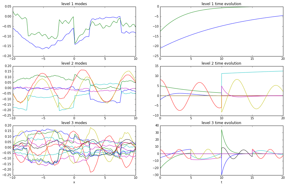
With the stitch command, we can extract all of the DMD modes and time evolutions from a given level into a single pair of \(\Phi\) and \(\Psi\) matrices. For example, here we pull out the \(\Phi\) and \(\Psi\) matrices from the first, second, and third levels. their plots are below.

Notice how the first level modes look like those we’d generate with a single application of the DMD. In contrast, the second and third levels show clear discontinuities at the instants in time where the data was split into two pieces. Note that only three levels are shown because the plots get very busy very quickly.

Phi0,Psi0 = stitch(nodes, 0)
Phi1,Psi1 = stitch(nodes, 1)
Phi2,Psi2 = stitch(nodes, 2)

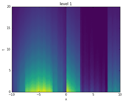
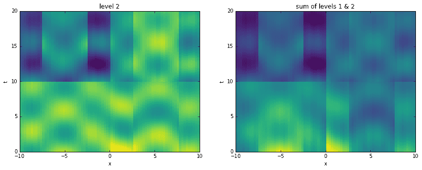
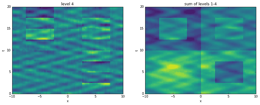
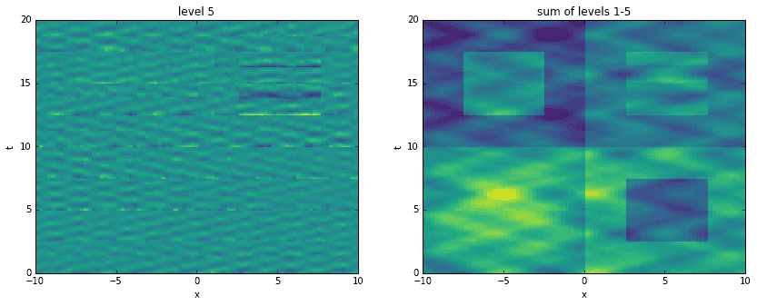
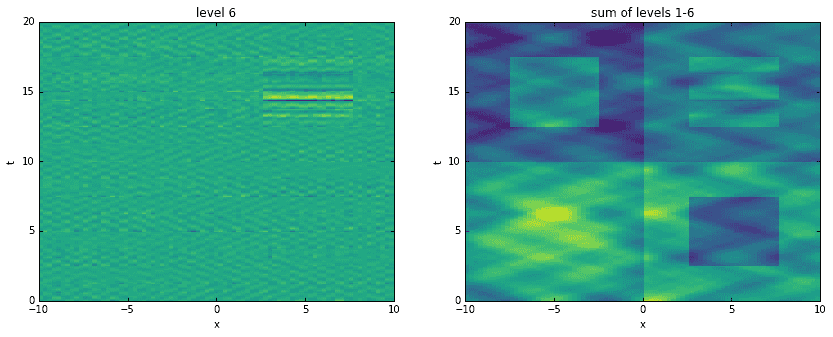
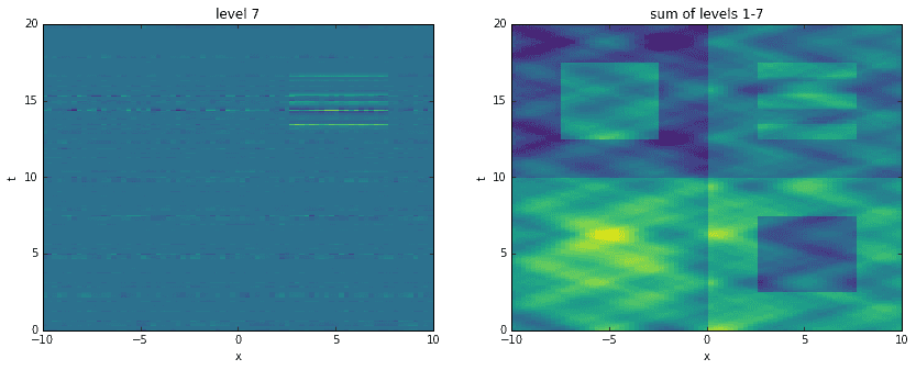
Going a step further, here we recreate the original data by adding levels together. For each level, starting with the first, we construct an approximation to the data at the corresponding time scale. Then, we sequentially add them all together, one on top of another. It is interesting to see how the original data has been broken into features of finer and finer resolution.

D_mrdmd = [dot(*stitch(nodes, i)) for i in range(7)]

Conclusion

The power of the mrDMD should be evident. First of all, it is self-contained, with no parameters to tweak — a big plus. Secondly, it allows us to extract features at different levels of resolution, thereby providing a principled way to identify long-, medium-, and short-term trends in data. It is able to cleanly handle transient phenomena and it removes noise without much added effort (especially when using the optimal SVHT). Lastly, it is efficient and general enough that it might be applied successfully in a wide variety disciplines (physics, biology, finance, etc.). The mrDMD is clearly a great addition to the scientist’s toolbox.

References

1. Kutz, J. Nathan, Xing Fu, and Steven L. Brunton. “Multiresolution Dynamic Mode Decomposition.” SIAM Journal on Applied Dynamical Systems 15.2 (2016): 713-735.
2. Jovanović, Mihailo R., Peter J. Schmid, and Joseph W. Nichols. “Sparsity-promoting dynamic mode decomposition.” Physics of Fluids (1994-present) 26.2 (2014): 024103.