A Crash Course using Meep

Meep is a versatile, free, and open-source software designed for electromagnetics simulations using the finite-difference time-domain (FDTD) method. Despite its extensive range of applications, broad features, and comprehensive documentation, new users might find it quite technical and challenging to learn.

In this beginner’s guide, we’ll recreate the famous double slit experiment in two dimensions, explaining the code at each step.

Environment Setup

First we must quickly setup a Python environment from which we can import and utilize Meep. While many methods exist for installing Meep, here we use Conda, which is probably the simplest way. For alternative installation methods, please refer to Meep’s official documentation.

To start, download and install Miniconda and choose an installation directory, for instance, ~/.miniconda3/. During installation, you’ll be prompted to initialize Miniconda. It’s recommended to select “yes”. This action will modify your .bashrc file (or similar), ensuring that Conda’s base environment is activated each time you open a new terminal.

If prefer not to have the base environment automatically activated, disable this feature issuing the following command from a fresh terminal:

conda config --set auto_activate_base false

You can manually activate the base environment using:

conda activate

We’ll use a Conda configuration file to create the environment. Copy and paste the following content into a file called environment.yml:

name: meep
channels:
  - conda-forge
  - defaults
dependencies:
  - python=3.11
  - matplotlib=3.7
  - numpy=1.25
  - opencv=4.7
  - pymeep=1.27.0
  - pymeep-extras=1.27.0

Then, to create the environment, run:

conda env create -f environment.yml

Finally, activate the newly created environment using:

conda activate meep

You are now ready to use Meep from Python.

Python Project

Launch Python and import the packages we’ll be using. Let me briefly explain what each package is for. The central focus of this post is, of course, meep, which will be performing all of the heavy lifting in our electromagnetics simulation. To manipulate and work with the data produced by these simulations, we’ll use numpy. Since our simulations can generate substantial data, we leverage h5py for efficient storage. We use pyplot for data visualization and plotting. Finally, os is used for handling various filesystem tasks.

import h5py
import matplotlib.pyplot as plt
import meep as mp
import numpy as np
import os

For convenience — and to avoid cluttering up the more important code — let’s also define some plotting functions now. We’ll use them later.

from matplotlib.colors import LinearSegmentedColormap

# Increase the default resolution for images
plt.rcParams['figure.dpi'] = 300
plt.rcParams['savefig.dpi'] = 300

# Plot everything on a dark background
plt.style.use('dark_background')

# Some custom colormaps
cmap_alpha = LinearSegmentedColormap.from_list(
    'custom_alpha', [[1, 1, 1, 0], [1, 1, 1, 1]])
cmap_blue = LinearSegmentedColormap.from_list(
    'custom_blue', [[0, 0, 0], [0, 0.66, 1], [1, 1, 1]])

def label_plot(ax, title=None, xlabel=None, ylabel=None, elapsed=None):
    """
    Add a title and x/y labels to the plot.
    """
    if title:
        ax.set_title(title)
    elif elapsed is not None:
        ax.set_title(f'{elapsed:0.1f} fs')
    if xlabel is not False:
        ax.set_xlabel('x (μm)'if xlabel is None else xlabel)
    if ylabel is not False:
        ax.set_ylabel('y (μm)'if ylabel is None else ylabel)

def plot_eps_data(eps_data, domain, ax=None, **kwargs):
    """
    Plot the wall geometry (dielectric data) within the domain.
    """
    ax = ax or plt.gca()
    ax.imshow(eps_data.T, cmap=cmap_alpha, extent=domain, origin='lower')
    label_plot(ax, **kwargs)

def plot_ez_data(ez_data, domain, ax=None, vmax=None, aspect=None, **kwargs):
    """
    Plot the amplitude of the complex-valued electric field
    data within the domain.
    """
    ax = ax or plt.gca()
    ax.imshow(
        np.abs(ez_data.T),
        interpolation='spline36',
        cmap=cmap_blue,
        extent=domain,
        vmax=vmax,
        aspect=aspect,
        origin='lower',
        )
    label_plot(ax, **kwargs)

def plot_pml(pml_thickness, domain, ax=None):
    ax = ax or plt.gca()
    x_start = domain[0] + pml_thickness
    x_end = domain[1] - pml_thickness
    y_start = domain[2] + pml_thickness
    y_end = domain[3] - pml_thickness
    rect = plt.Rectangle(
        (x_start, y_start),
        x_end - x_start,
        y_end - y_start,
        fill=None,
        color='#fff',
        linestyle='dashed',
        )
    ax.add_patch(rect)

Meep Units

Before going any further with the code, there’s an essential high-level concept that should be well-understood. Meep’s functionality stems from Maxwell’s equations, which are scale-invariant. Consequently, Meep employs dimensionless units.

Practically, this flexibility allows you to define the spatial and temporal dimensions of your simulation in any way you prefer. However, it also necessitates a careful conversion of any dimension-specific values into “Meep units” before using them as arguments in Meep’s various classes.

For the purposes of this post, let’s define the dimensions as follows:

• Lengths are measured in micrometers (μm)
• Time is measured in femtoseconds (fs)

Meep defines the speed of light internally as unity. Consequently, the units of distance and time in Meep both equate to 1 μm. A simple way to think about it is that one Meep time unit is how long it takes for light to traverse one Meep unit of distance.

For converting time from fs to Meep units, defining the speed of light in μm/fs is beneficial. So,

Therefore, time \(t\) measured in fs is equivalent to approximately \(0.3t\) in Meep time units. This conversion will be useful later.

Domain & Geometry

The following piece of code first defines the speed of light (SOL) in units of μm per fs. Then, it sets up the 2-dimensional spatial domain for the simulation, specified in μm. The domain list represents the extent of the domain, and the center and cell_size variables define the center point and size of the cell in this domain, respectively, using Meep’s Vector3 object. These parameters will be used in the subsequent steps of the simulation.

# The speed of light in μm/fs
SOL = 299792458e-9

# 2D spatial domain measured in μm
domain = [0, 30, -10, 10]
center = mp.Vector3(
    (domain[1] + domain[0]) / 2,
    (domain[3] + domain[2]) / 2,
    )
cell_size = mp.Vector3(
    domain[1] - domain[0],
    domain[3] - domain[2],
    )

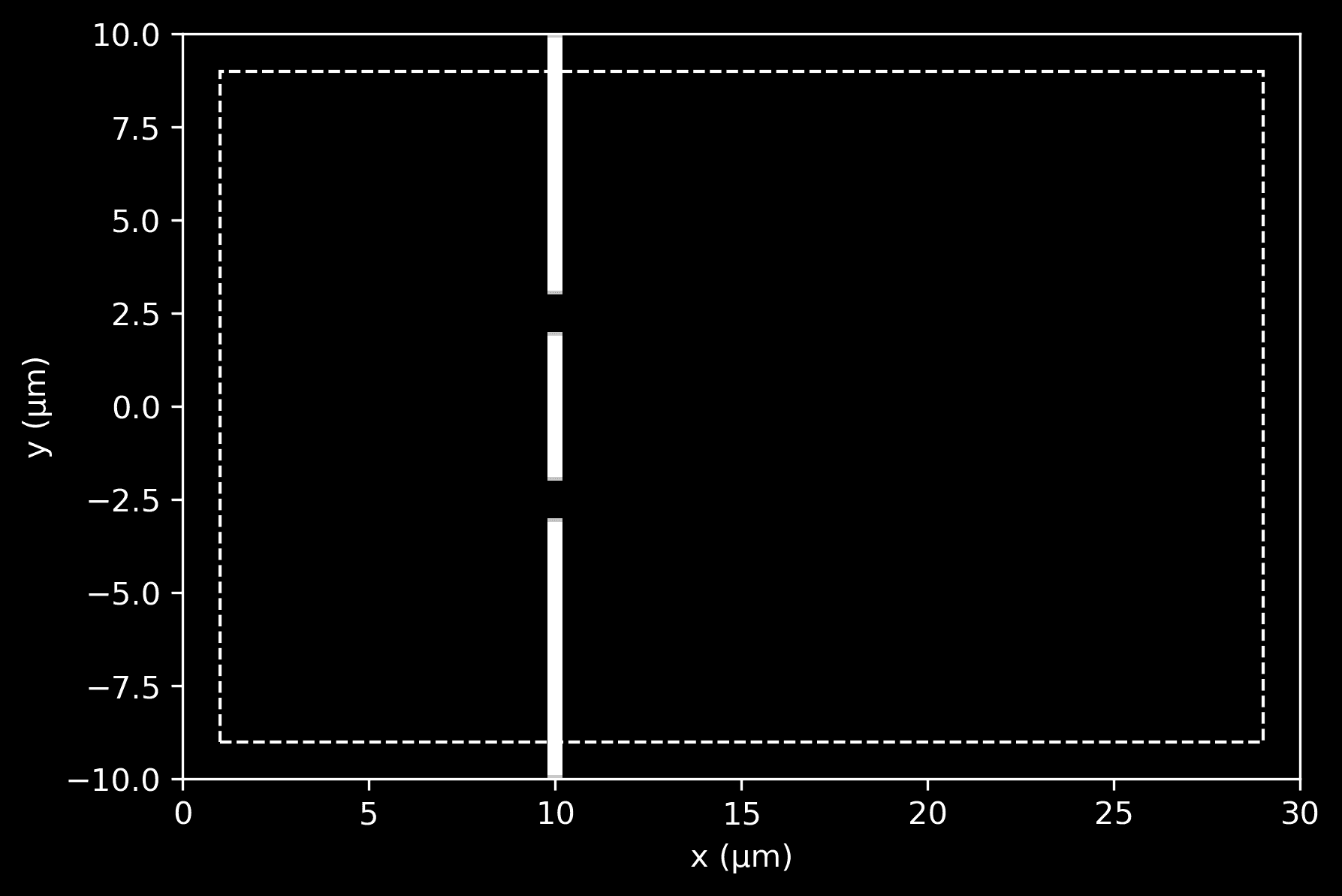
The next code segment defines a wall with two apertures (holes). The wall’s dimensions and position, along with the size of the apertures, are all defined. The wall is constituted by three blocks arranged vertically and is created using a material with an exceptionally high dielectric constant, effectively blocking and reflecting light instead of allowing it to pass through.

The blocks are aligned to create the double-slit configuration with two outer blocks representing the edges of the wall and an inner block separating the two apertures. The geometry of the wall is created using these block definitions.

Moreover, the code sets up perfectly matched layers (PML) for the simulation boundaries. The PML is a layer that surrounds the simulation cell and is designed to absorb all incident waves without any reflection, thereby mimicking an infinite space.

# Dimensions of wall with two apertures
wall_position = 10
wall_thickness = 0.5
aperture_width = 1
inner_wall_len = 4  # wall separating the apertures
outer_wall_len = (
    cell_size[1]
    - 2*aperture_width
    - inner_wall_len
    ) / 2

# Define a wall material with high dielectric constant,
# effectively blocking light and reflecting it instead
material = mp.Medium(epsilon=1e6)

# Define the wall as an array of 3 blocks arranged vertically
geometry = [
    mp.Block(
        mp.Vector3(wall_thickness, outer_wall_len, mp.inf),
        center=mp.Vector3(
            wall_position - center.x,
            domain[3] - outer_wall_len / 2),
        material=material),
    mp.Block(
        mp.Vector3(wall_thickness, outer_wall_len, mp.inf),
        center=mp.Vector3(
            wall_position - center.x,
            domain[2] + outer_wall_len / 2),
        material=material),
    mp.Block(
        mp.Vector3(wall_thickness, inner_wall_len, mp.inf),
        center=mp.Vector3(wall_position - center.x, 0),
        material=material),
    ]

# Perfectly matched layer of thickness 1
pml_thickness = 1
pml_layers = [mp.PML(pml_thickness)]

To quickly visualize the wall geometry, initialize a simulation (without running it) and extract the dielectric data.

# Extract and visualize the dielectric data (wall geometry)
sim = mp.Simulation(cell_size=cell_size, geometry=geometry, resolution=10)
sim.init_sim()
eps_data = sim.get_array(center=mp.Vector3(), size=cell_size, component=mp.Dielectric)
ax = plt.gca()
plot_pml(pml_thickness, domain, ax=ax)
plot_eps_data(eps_data, domain, ax=ax)

Light Source

Next we define a light source with properties similar to a laser. We choose a wavelength of 470 nanometers, which corresponds approximately to light blue visible light, and a beam width of 6 units. The frequency of the light source is calculated as the reciprocal of the wavelength, given that the speed of light in Meep units is one.

# Light wavelength, frequency, and beam width
source_lambda = 0.47  # in μm
source_frequency = 1 / source_lambda
source_beam_width = 6

To approximate a laser, we want to design a continuous Gaussian beam that originates from the left-hand side and propagates towards the right. Ideally, this beam should be collimated, which means that the light rays are parallel to each other, resulting in a beam that doesn’t spread out and maintains its narrow shape over distance. Unfortunately, achieving this setup is a somewhat involved, as Meep does not offer a built-in source that fulfills these requirements directly. At first glance, the GaussianBeam2DSource may seem like what we want, but it requires a focal point, thus it isn’t truly collimated.

To overcome this, we will combine Meep’s various source classes with our own amplitude function, which simply returns a complex current amplitude for any given position. Let’s start the process of building our light source by constructing this function.

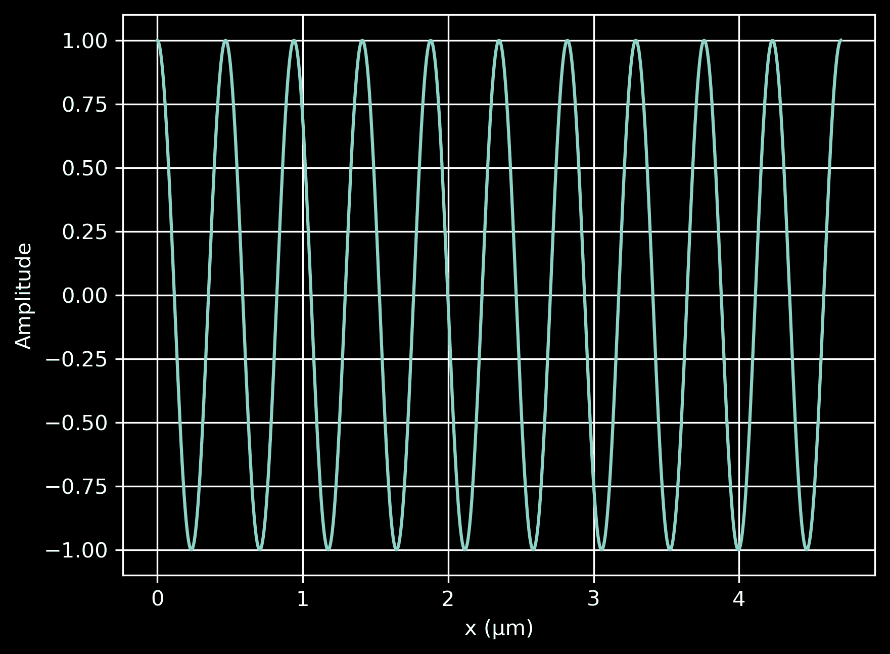
First, we define a function that returns a complex-valued plane wave propagating in the \(x\)-direction. This function uses the np.exp function to generate the complex exponential, which is representative of a wave. The plot we create here shows the real part of the wave amplitude as a function of position, illustrating how it propagates along the \(x\)-axis, regardless of \(y\). The wave amplitude varies sinusoidally with \(x\), as expected.

# A method to return a complex-valued plane wave in the x-direction
def plane_wave(x):
    return np.exp(2j * np.pi / source_lambda * x)

# Plot the plane wave
xarr = np.linspace(0, 10*source_lambda, 1000)
wave = plane_wave(xarr)
plt.plot(xarr, wave.real)
plt.xlabel('x (μm)')
plt.ylabel('Amplitude')
plt.grid(True)

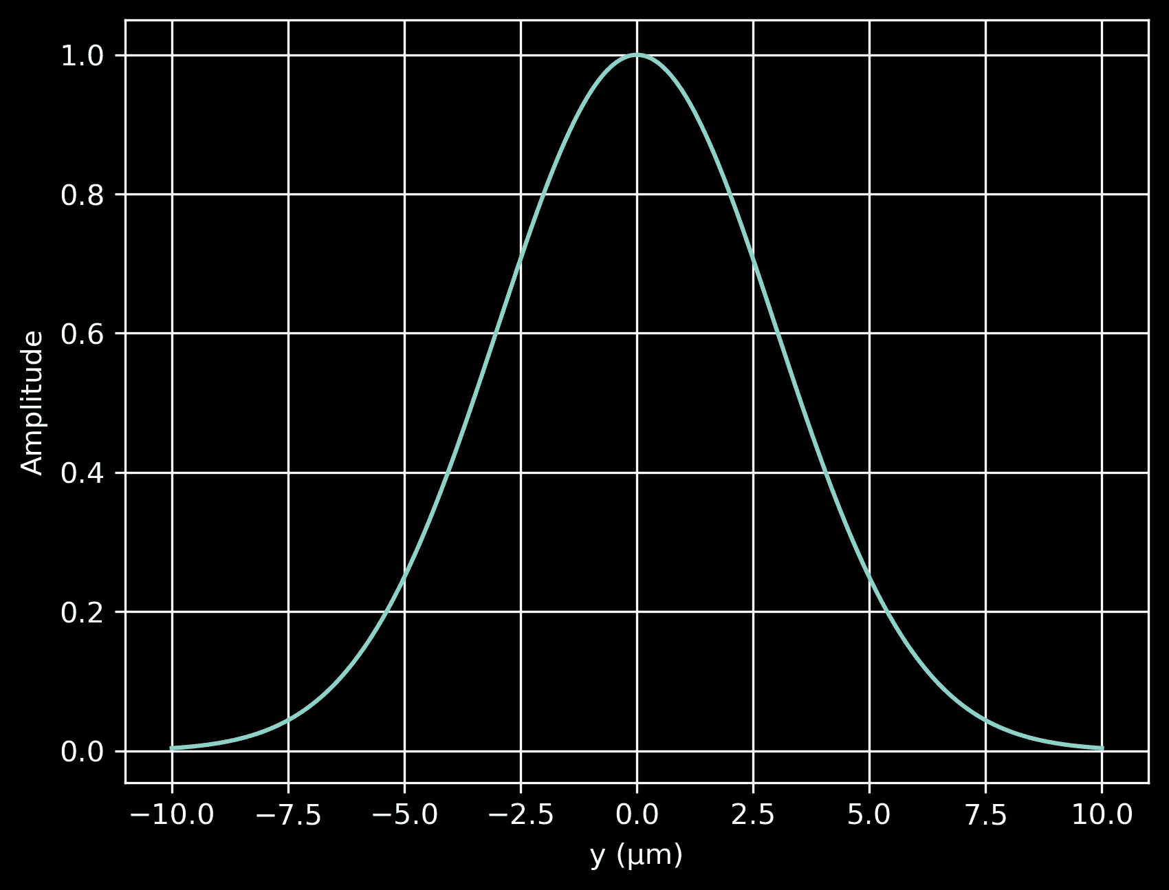
Next, we define another function to compute the Gaussian profile along the \(y\)-direction. This profile decreases from a maximum at \(y=0\) (the beam center) to near-zero values as we move away from the center in either direction. The width of the Gaussian profile is determined by source_beam_width / 2, representing the standard deviation of the Gaussian distribution. This profile is essentially a cross-sectional distribution of the beam amplitude. When we plot the profile, we see that it has a peak at \(y=0\) and falls off on either side, illustrating how the intensity of the laser light decreases away from the center of the beam.

# A method to compute the Gaussian profile in the y-direction
def gaussian_profile(y):
    return np.exp(-y**2 / (2 * (source_beam_width / 2)**2))

# Plot the Guassian profile
yarr = np.linspace(domain[2], domain[3], 200)
prof = gaussian_profile(yarr)
plt.plot(yarr, prof)
plt.xlabel('y (μm)')
plt.ylabel('Amplitude')
plt.grid(True)

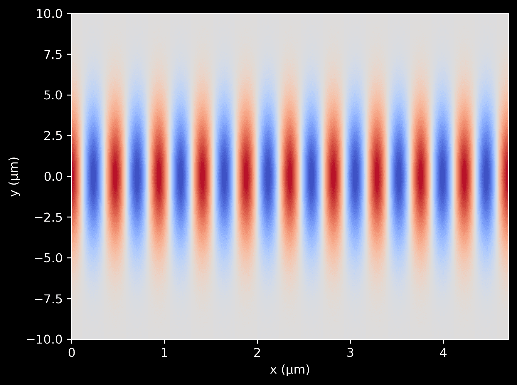
Now we can combine the two functions defined above to generate a complex amplitude distribution for a 2D Gaussian beam. This is achieved by multiplying the plane wave function by the Gaussian profile function. The resulting function gives the complex amplitude of the light wave at any position \((x, y)\) in the domain. We can plot it as a color-map, showing the spatial variation of the beam intensity in the 2D plane.

# A 2D grid of points
X, Y = np.meshgrid(xarr, yarr)

# Plot the combined terms
combined = plane_wave(X) * gaussian_profile(Y)
plt.imshow(
    np.real(combined),
    cmap='coolwarm',
    aspect='auto',
    extent=[xarr[0], xarr[-1], yarr[0], yarr[-1]],
    origin='lower',
    )
plt.xlabel('x (μm)')
plt.ylabel('y (μm)')

We use the combined function from the previous step to define a light source in Meep. This is achieved using Meep’s Source object, to which we provide a ContinuousSource configured to our specific frequency. We specify the direction and type of the current component with mp.Ez. Using center and size we position the source to span the entire length of the left-hand edge of the domain, leaving some extra room for the PML on the left. Importantly, the amp_func parameter is given the combined function we defined above, which ensures that the light source has the desired spatial amplitude variation.

Since our light source extends into the PML regions on the top and bottom, it’s useful to set is_integrated=True. This helps to correctly handle the source’s overlap with the PML, minimizing any undesirable interference effects at the boundary.

Lastly, a note about the frequency supplied to the ContinuousSource object and the source_lambda supplied to the amp_func method: while they are related (since wavelength and frequency are inversely related in light waves), they control different aspects of the source. The frequency sets the temporal oscillation of the source, i.e., how fast it’s oscillating in time. On the other hand, source_lambda in amp_func helps set up the initial spatial phase distribution across the source plane. Both are necessary to properly define the source’s temporal and spatial characteristics.

def amp_func(pos):
    return plane_wave(pos[0]) * gaussian_profile(pos[1])

source = mp.Source(
    src=mp.ContinuousSource(
        frequency=source_frequency,
        is_integrated=True,
        ),
    component=mp.Ez,
    center= mp.Vector3(1, 0, 0) - center,  # positioned far-left, excluding PML
    size=mp.Vector3(y=cell_size[1]),       # span entire height, including PML
    amp_func=amp_func,
    )

Simulation

Now we can finally construct and run the simulation. We’ll start by defining an appropriate resolution for the simulation.

In Meep, the resolution parameter in the Simulation class determines the spatial discretization of the simulation domain. Higher resolution means more grid points per unit length and thus more detailed representation of the geometry and fields, but it also means a larger problem size, leading to longer simulation time and greater memory usage.

Here are some guidelines to choose a suitable resolution:

1. Wavelength of the light: The grid size should be small compared to the smallest wavelength in the simulation. A good rule of thumb is to have at least 8-10 pixels per smallest wavelength. For example, if the smallest wavelength of interest is 0.5 μm, a resolution of 16-20 pixels/μm could be a good starting point.

2. Feature size of the structures: The resolution should be high enough to accurately describe the smallest geometric features of the structure in your simulation. If you have small, intricate details in your geometry, you’ll need a higher resolution to accurately capture these.

3. Simulation time and resources: The resolution you choose also depends on how much computation resources you have and how long you’re willing to wait. Higher resolution will increase both the computation time and memory requirements.

4. Accuracy vs efficiency trade-off: Start with a moderate resolution, run the simulation, and analyze the results. Then increase the resolution and repeat. If the results change significantly with increasing resolution, it might be an indication that the initial resolution was too low. Once the results converge (i.e., further increases in resolution result in negligible changes in the results), you’ve found a resolution that’s high enough for your needs.

For our simple scenario we’ll limit ourselves to the first two guidelines. First identify the smallest feature length or wavelength. Then assign 10 pixels to that length to determine the simulation resolution. Rounding up to the nearest integer ensures that the grid volume has an integer number of pixels.

# Define resolution in terms of smallest component
smallest_length = min(
    source_lambda,
    wall_thickness,
    aperture_width,
    inner_wall_len,
)
pixel_count = 10
resolution = int(np.ceil(pixel_count / smallest_length))
print('Simulation resolution:', resolution)

Output:

Simulation resolution: 22

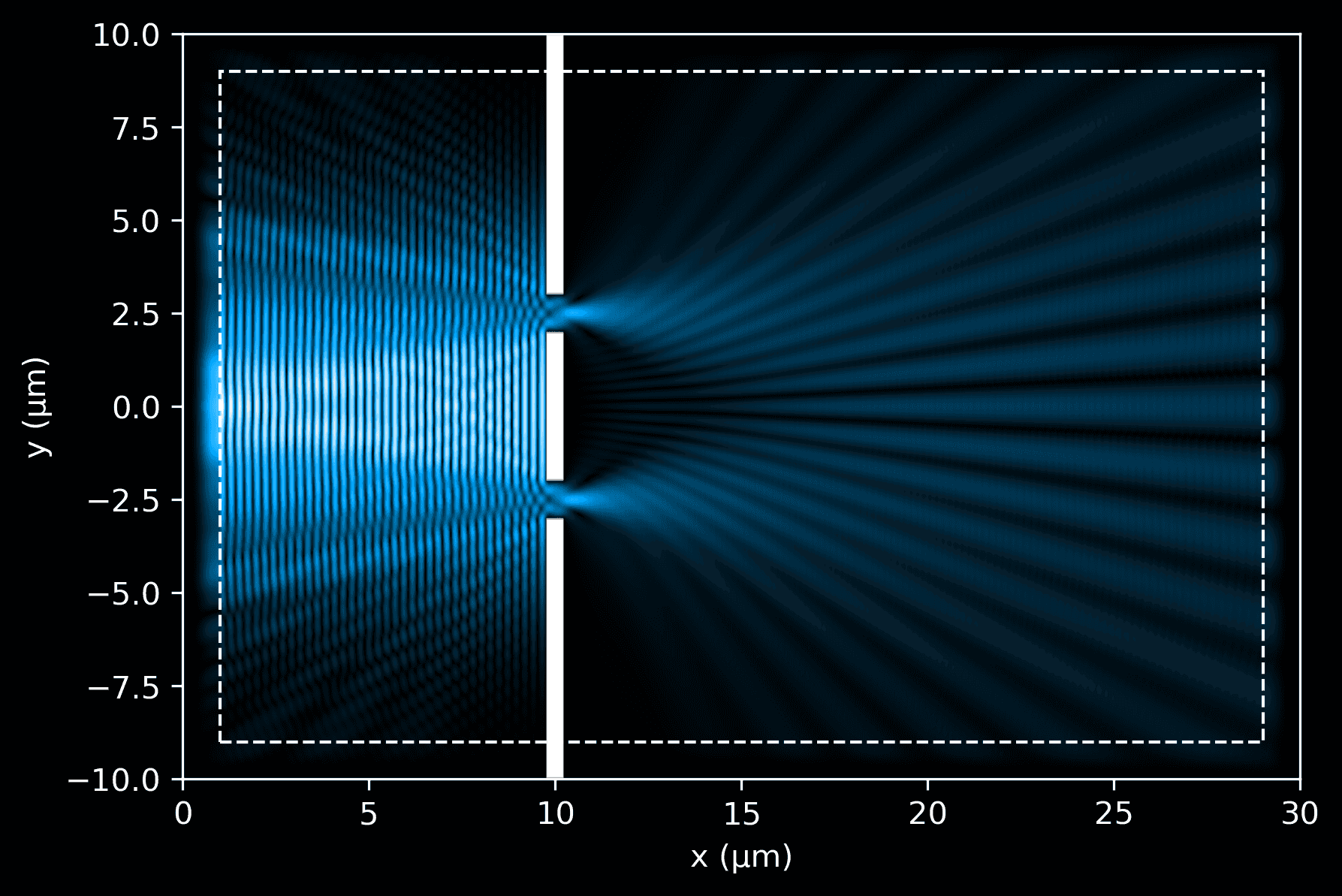
Now create a Simulation object, pulling together the variables we defined earlier, such as cell size, light source, boundary layers, geometry, and resolution. Also specify force_complex_fields=True, forcing Meep to use complex-valued fields rather than real-valued.

Once the setup is complete, run the simulation for a duration slightly exceeding the time it would take for light to travel across the full length of the domain. This additional time is necessary to allow any initial wavefront disturbances to exit the simulation area, thereby cleaning up the final result.

Finally, extract the data from the completed simulation, and use our plotting functions to visualize it. We can now see how the electric field interacts with the geometry objects.

# Simulation object
sim = mp.Simulation(
    cell_size=cell_size,
    sources=[source],
    boundary_layers=pml_layers,
    geometry=geometry,
    resolution=resolution,
    force_complex_fields=True,
    )

# Convenience method to extract Ez and dielectric data
def get_data(sim, cell_size):
    ez_data = sim.get_array(
        center=mp.Vector3(), size=cell_size, component=mp.Ez)
    eps_data = sim.get_array(
        center=mp.Vector3(), size=cell_size, component=mp.Dielectric)
    return ez_data, eps_data
    
# Run simulation until light travels full length (plus some)
sim.run(until=cell_size[0] + 10)
ez_data, eps_data = get_data(sim, cell_size)

# Plot simulation
ax = plt.gca()
plot_ez_data(ez_data, domain, ax=ax)
plot_eps_data(eps_data, domain, ax=ax)
plot_pml(pml_thickness, domain, ax=ax)

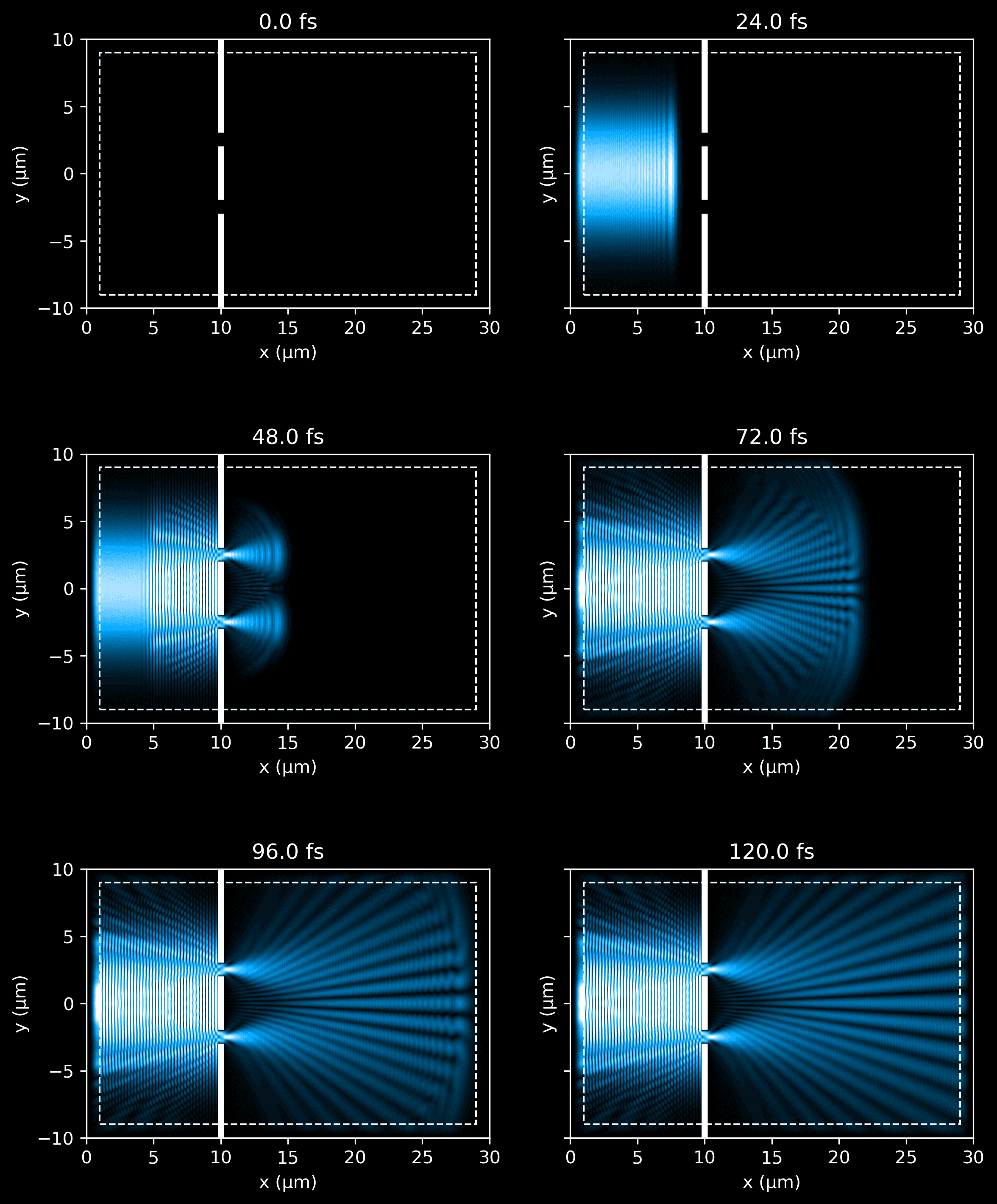
In the next code block, we organize and run a simulation over a defined period, given in fs, capturing periodic snapshots of the process. These frames provide a time-resolved picture of how the light travels through the simulated domain. Keep in mind that we must convert into Meep time units by multiplying by SOL, ensuring that our simulation aligns with the dimensional units used by the Meep framework.

The data generated during this simulation is saved in an efficient binary format, ideal for handling large datasets. This allows us to execute the simulation in one go, capturing the entire process without interruption, while also optimizing our computational resources.

For convenience and cleaner code, we’re creating a reusable wrapper function, simulate, which handles the entire operation from start to finish. It prepares the data storage, runs the simulation in intervals, and saves the electric field data for each snapshot.

# Sim duration and number of snapshots
sim_time = 120  # in fs
n_frames = 6

# Where to save the results
sim_path = 'simulation.h5'

# Simulation object
sim = mp.Simulation(
    cell_size=cell_size,
    sources=[source],
    boundary_layers=pml_layers,
    geometry=geometry,
    resolution=resolution,
    force_complex_fields=True,
    )

def simulate(sim, sim_path, sim_time, n_frames):
    
    # Remove previous sim file, if any
    if os.path.exists(sim_path):
        os.remove(sim_path)

    # Time delta (in fs) between snapshots. Note that
    # we subtract 1 because we include the initial state
    # as the first frame.
    fs_delta = sim_time / (n_frames - 1)
    
    # Save data to an HDF5 binary file
    with h5py.File(sim_path, 'a') as f:
    
        # Save simulation params for future reference
        f.attrs['sim_time'] = sim_time
        f.attrs['n_frames'] = n_frames
        f.attrs['fs_delta'] = fs_delta
        f.attrs['resolution'] = sim.resolution
        
        # Save initial state as first frame
        sim.init_sim()
        ez_data, eps_data = get_data(sim, cell_size)
        f.create_dataset(
            'ez_data',
            shape=(n_frames, *ez_data.shape),
            dtype=ez_data.dtype,
            )
        f.create_dataset(
            'eps_data',
            shape=eps_data.shape,
            dtype=eps_data.dtype,
            )
        f['ez_data'][0]  = ez_data
        f['eps_data'][:] = eps_data
    
        # Simulate and capture remaining snapshots
        for i in range(1, n_frames):
    
            # Run until the next frame time
            sim.run(until=SOL * fs_delta)
    
            # Capture electral field data    
            ez_data, _ = get_data(sim, cell_size)
            f['ez_data'][i]  = ez_data

simulate(sim, sim_path, sim_time, n_frames)

When the simulation completes, visualize the snapshots side-by-side.

fig_rows = 3
fig_cols = 2
n_subplots = fig_rows * fig_cols
fig, ax = plt.subplots(
    fig_rows,
    fig_cols,
    figsize=(9, 12),
    sharex=False,
    sharey=True,
    )

with h5py.File(sim_path, 'r') as f:
    for k in range(n_subplots):
        i, j = int(k / fig_cols), (k % fig_cols)
        # i, j = (k % fig_rows), int(k / fig_rows)
        _ax = ax[i][j]
        ez_data = f['ez_data'][k]
        eps_data = f['eps_data'][:]
        elapsed = k * f.attrs['fs_delta']
        vmax = 0.6  # force consistent brightness
        plot_ez_data(ez_data, domain, ax=_ax, vmax=vmax, elapsed=elapsed)
        plot_eps_data(eps_data, domain, ax=_ax)
        plot_pml(pml_thickness, domain, ax=_ax)

Interference Patterns

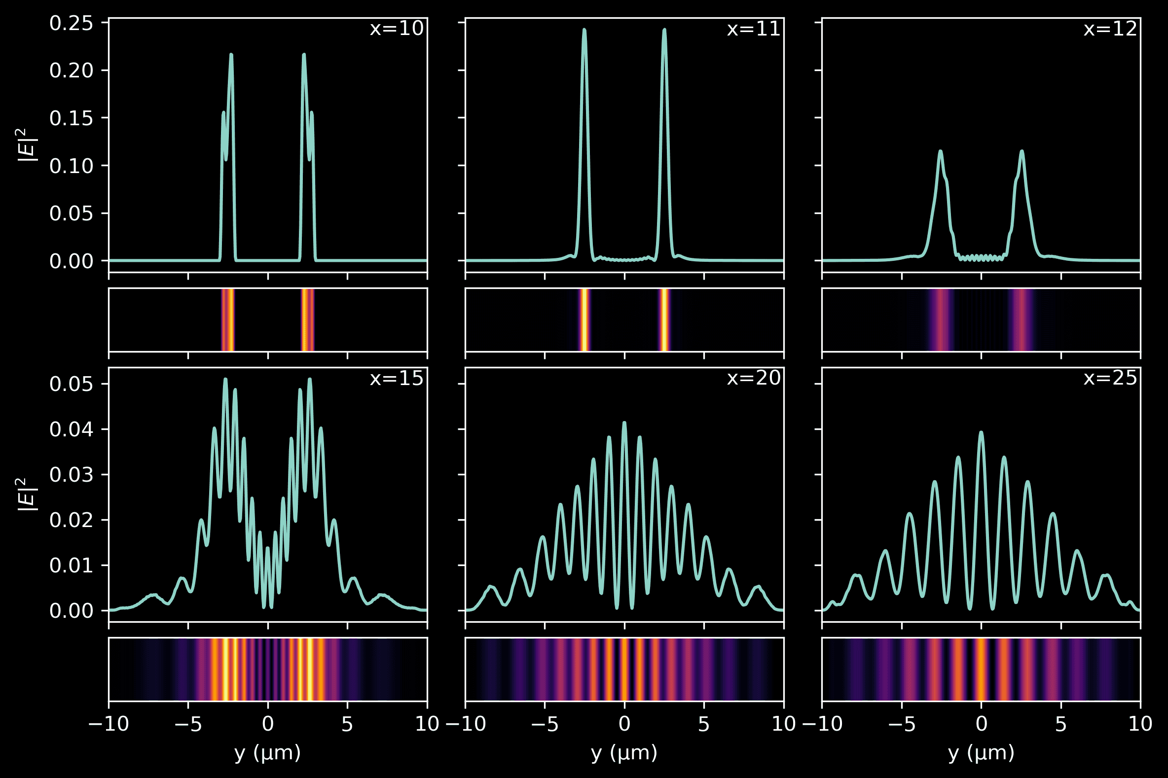
For the final part of the tutorial, we are focusing on the visualization of the interference pattern created when light exits the double slits. By doing so, we can better understand how the interference pattern evolves as the light propagates further away from the slits. Keep in mind that the intensity of a wave is proportional to the square of its amplitude

Utilizing the final snapshot from our simulation — which offers the most “complete” view of the propagated light and has fewer residual ripples — we compute the light intensity at various slices along the \(x\)-axis, following the light’s exit from the double slits. Each slice provides us with an instantaneous snapshot of the light intensity at that distance, illustrating the evolving interference pattern.

# Grab final simulation snapshot without time-averaging
with h5py.File(sim_path, 'r') as f:
    final_snap = f['ez_data'][-1]

# Compute intensity as square of the complex amplitude
final_snap = np.abs(final_snap)**2

# Pick slices at different distances from the double slit
slice_dists = [10, 11, 12, 15, 20, 25]
slices = [final_snap[i * resolution] for i in slice_dists]
yarr = np.linspace(domain[2], domain[3], final_snap.shape[1])

# A rather involved plotting function
def plot_intensity(slice, yarr, ax1, ax2, vmax=None, xval=None, xlabel=False, ylabel=False):
    ax1.plot(yarr, slice)
    ax1.tick_params(axis='x', labelbottom=False)
    if ylabel:
        ax1.set_ylabel('$|E|^2$')
    else:
        ax1.tick_params('y', labelleft=False)
    if xval:
        ax1.annotate(
            f'x={xval}',
            xy=(1, 1),
            xytext=(-4, -4),
            xycoords='axes fraction',
            textcoords='offset pixels',
            horizontalalignment='right',
            verticalalignment='top',
            )
    ax2.imshow(
        np.vstack(slice).T,
        cmap='inferno',
        aspect='auto',
        vmax=vmax,
        extent=[yarr[0], yarr[-1], 0, 1],
        )
    ax2.set_xlim([yarr[0], yarr[-1]])
    ax2.tick_params('y', labelleft=False)
    ax2.set_yticks([])
    if xlabel:
        ax2.set_xlabel('y (μm)')
    else:
        ax2.tick_params(axis='x', labelbottom=False)

fig, ax = plt.subplots(
    4, 3,
    figsize=(9, 6),
    gridspec_kw=dict(
        width_ratios=(4, 4, 4),
        height_ratios=(4, 1, 4, 1),
        wspace=0.12,
        hspace=0.1,
        ),
    sharex='col',
    sharey='row',
    )
for k, slice in enumerate(slices):
    i = 2 * int(k / 3)
    j = k % 3
    plot_intensity(
        slice, yarr, ax[i][j], ax[i+1][j],
        vmax=np.max(slices[:3]) if k < 3 else np.max(slices[3:]),
        xval=slice_dists[k],
        xlabel=(i==2),
        ylabel=(j==0))

Summary

That concludes the tutorial — I hope it has proven useful to you! The aim was to create an accessible, beginner’s guide to electromagnetics simulation using Meep, a free, open-source software built on the finite-difference time-domain (FDTD) method. We began by setting up the Python environment and importing the required packages. Then, we delved into the heart of the tutorial, recreating the iconic double-slit experiment. We covered key concepts such as Meep units, domain and geometry setup, light source creation, and simulation execution, using sample code for better understanding. We finished by exploring interference patterns, thereby showcasing Meep’s capabilities in visualizing and comprehending complex electromagnetics phenomena.

Resources