Investigating the Lorenz attractor

Chaotic Attractor

The Lorenz attractor is a very well-known phenomenon of nature that arises out a fairly simple system of equations. Discovered in the 1960’s by Edward Lorenz, this system is one of the earliest examples of chaos. Lorenz referred to the chaotic dynamics he witnessed as the “butterfly effect”. Essentially, this means that the system has huge sensitivity to initial conditions.

What is sensitivity to initial conditions? Well, it’s the idea that small — even minuscule — displacements between any two initial states of the system will cause widely diverging mid- to long-term behavior. So, if you pick any pair of super-close points in the state space governed by the Lorenz equations and simulate them forward, they will not stay together! Check out this video I made as an undergraduate for an independent study on chaos theory. It explains the idea in a more visual way.

Notice how the three colors start out right on top of each other. Then, suddenly, they fan out into totally different directions! That is an example of chaos. However, the really peculiar thing is that, no matter where you place your initial point, its trajectory seems to ultimately create/ follow a cool butterfly formation. We call this formation an attractor. More accurately, it is a strange attractor — meaning that the attracting set has a fractal geometry. For more information on chaos, fractals, and strangeness, you can read an undergraduate paper I published about the “big picture” behind chaos theory: Attractors: Nonstrange to Chaotic. Disclaimer: I was very new to the subject when I wrote it, so there might be errors and inconsistencies. Fact check!

Lorenz Equations

The Lorenz equations are as follows:

\(\dot x = \sigma(y-x)\)

\(\dot y = x(\rho-z)-y\)

\(\dot z = xy-\beta z\)

Where \(\sigma\) is the Prandtl number, \(\rho\) is the Rayleigh number divided by the critical Rayleigh number, and \(\beta\) is a geometric factor. However, in most case that I’ve seen of people investigating the Lorenz system, these constants are assigned particular values:

\(\sigma=10\)

\(\rho=28\)

\(\beta= 8/3\)

Using some basic algebra, we can find the fixed points of the system (\(x\)-\(y\)-\(z\) coordinates at which a particle’s position never changes). Simply set \(\dot x=\dot y=\dot z= 0\) and solve for \(x\), \(y\), and \(z\). The fixed points are:

\(P^*_0=(0,0,0)\)

\(P^*_1=\left(\sqrt{b(r-1)}, \sqrt{b(r-1)}, r-1\right)\)

\(P^*_2=\left(-\sqrt{b(r-1)}, -\sqrt{b(r-1)}, r-1\right)\)

Simulation

One of the best ways to understand this system is through simulation. My language of choice is Python, but you can integrate the equations in just about any language available. Below, I’ve written some scripts for simulating and plotting the system in both Python and Matlab. They both employ the Runge-Kutta integration method of order 4-5. Enjoy!

Python

First, make sure you’ve got SciPy, NumPy, and matplotlib installed. Then, just copy the code to a new file and execute at the command line. Note: It should work fine in both Python 2 and 3.

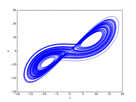
#!/usr/bin/env python

import numpy as np
from scipy.integrate import ode
import matplotlib.pyplot as plt

def lorenz(t, y, sig = 10, rho = 28, beta = 8/3):
    """The right hand side of the Lorenz attractor system."""

    return [
        sig * (y[1] - y[0]),
        y[0] * (rho - y[2]) - y[1],
        y[0] * y[1] - beta * y[2],
        ]

def main():
    """The main program."""

    # create arrays and set initial condition
    tspan = np.arange(0, 100, 0.01)
    Y = np.empty((3, tspan.size))
    Y[:, 0] = [1.5961, 0.1859, 4.7297] # random (x,y,z)

    # create explicit Runge-Kutta integrator of order (4)5
    r = ode(lorenz).set_integrator('dopri5')
    r.set_initial_value(Y[:, 0], tspan[0])

    # run the integration
    for i, t in enumerate(tspan):
        if not r.successful():
            break
        if i == 0:
            continue # skip the initial position
        r.integrate(t)
        Y[:, i] = r.y

    # plot the result in x-y plane
    plt.plot(Y[0, :], Y[1, :])
    plt.xlabel('x')
    plt.ylabel('y')
    plt.show()

if __name__ == '__main__':
    main()

The script will produce a plot in the \(x\)-\(y\) plane like this:

Matlab

Simply copy the following code to a new m file and execute in Matlab.

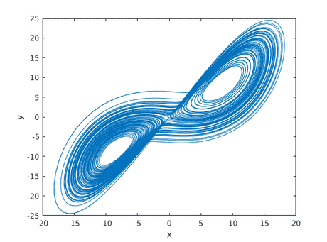
close all; clear; clc;

% set the domain and constants
tspan = 0:0.01:99.99;
sig = 10;
rho = 28;
beta = 8/3;

% the right hand side of the Lorenz attractor system
lorenz = @(t, y, sig, rho, beta) ([
    sig * (y(2) - y(1));
    y(1) * (rho - y(3)) - y(2);
    y(1) * y(2) - beta * y(3)]);

% run the integration
y0 = [1.5961; 0.1859; 4.7297]; % random (x,y,z)
[T, Y] = ode45(@(t, y) lorenz(t, y, sig, rho, beta), tspan, y0);
Y = Y(100:size(Y,1),:);

% plot the result in x-y plane
figure;
plot(Y(:,1), Y(:,2));
xlabel('x');
ylabel('y');

Matlab will produce a plot in the \(x\)-\(y\) plane like this:

References

1. Weisstein, Eric W. “Lorenz Attractor.” From MathWorld—A Wolfram Web Resource. http://mathworld.wolfram.com/LorenzAttractor.html