This post gives a brief example of how to apply the Kalman Filter (KF) and Extended Kalman Filter (EKF) Algorithms to assimilate “live” data into a predictive model. We set up an artificial scenario with generated data in Python for the purpose of illustrating the core techniques. The scenario involves multi-dimensional data, so the Kalman Equations are employed in their vector form.
Scenario: Biking at the Park
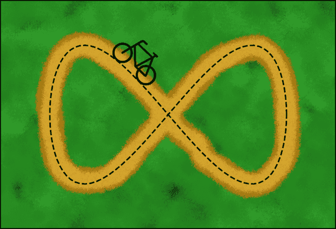
Imagine someone riding a bike at the park. The bike circuit forms a figure-eight that can be modelled with the equations:
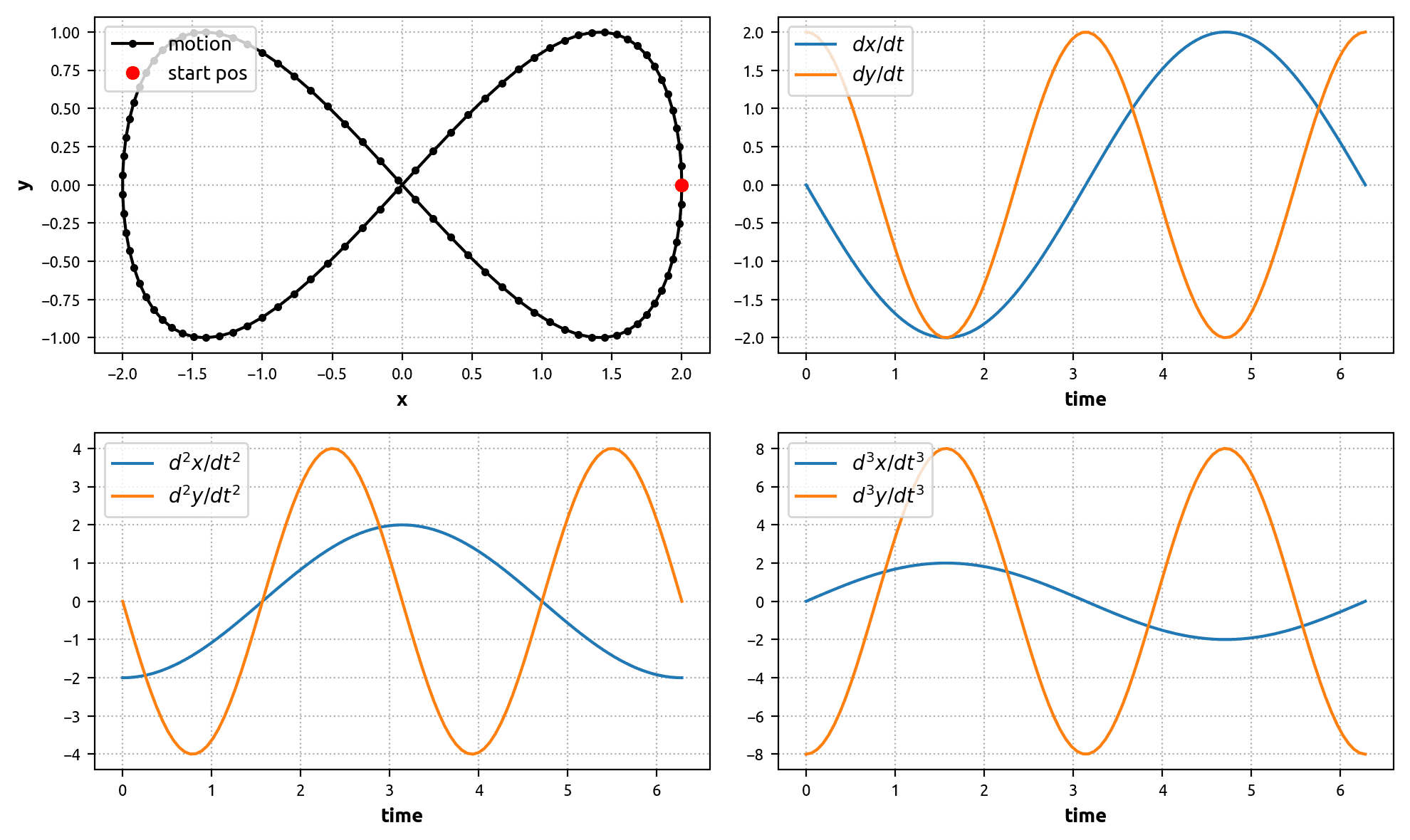
Consequently, the bike’s first, second, and third derivatives (velocity, acceleration, and jerk) are given by the equations:
In Python:
import numpy as npfrom numpy import pi, cos, sin, sqrt, diagfrom numpy.linalg import invfrom numpy.random import randnt = np.linspace(0, 2*pi, 100)dt = t[1] - t[0]# positionx = 2*cos(t)y = sin(2*t)# velocitydxdt = -2*sin(t)dydt = 2*cos(2*t)# acceld2xdt2 = -2*cos(t)d2ydt2 = -4*sin(2*t)# jerkd3xdt3 = 2*sin(t)d3ydt3 = -8*cos(2*t)
In this exercise, we are interested in accurately estimating the bike’s motion through time. Ideally, the method of estimation would assimilate as much information as is available to achieve the best results. There are a number of tools at our disposal to accomplish this.
Our first tool is a predictive model based on Newtonian physics. Given some knowledge or an estimate of the current position, velocity, and acceleration of the bike, we can apply the laws of motion to make a prediction of where the bike will be next. The predictive model might be written thus:
where \(t_m\) is the \(m\)-th time step and where the higher-order terms (including the jerk) are assumed to be zero-mean Gaussian signals \(J_x\) and \(J_y\). This model allows us to take the current state and predict a future state. The predictive model’s biggest flaw is that, given state information at time \(t_{m-1}\), it can only reasonably be expected to predict the state a couple time-step into the future (for example, at time \(t_m\)). Anything more than that and the predictions will likely diverge severely from the true solution due to dynamics in the higher-order terms and errors associated with the time-stepping.
This brings us to the second tool at our disposal: observation. Observation allows us to keep our predictive model up-to-date with the latest knowledge of the system state. But how do we observe the bike? It is assumed that the bike has sensors installed to provide three methods of motion measurement:
- A GPS device to estimate the current physical position of the bike.
- A speedometer to estimate the current speed of the bike.
- A gyroscope to estimate the current angular speed of the bike.
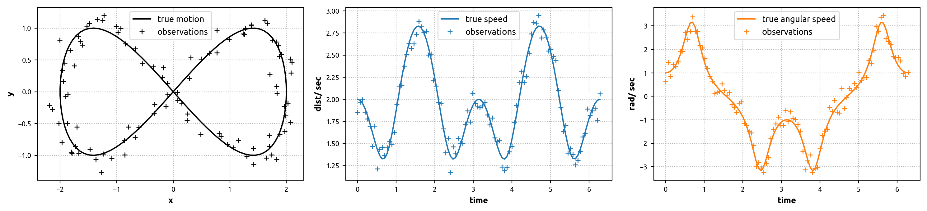
This measurement data can be used to greatly enhance our Newtonian prediction model (via the Kalman Filter). Given that the true speed (\(s\)) and true angular speed (\(\omega\)) of the bike as it moves around the figure-eight are calculated by the following equations, we have:
However, it is very reasonable to assume that the output of each of these sensors contains error. The Python code below shows how to generate noisy GPS, speedometer, and gyroscope signals.
# angular speed (scalar)omega = (dxdt*d2ydt2 - dydt*d2xdt2) / (dxdt**2 + dydt**2)# speed (scalar)speed = sqrt(dxdt**2 + dydt**2)# measurement errorgps_sig = 0.1omega_sig = 0.3speed_sig = 0.1# noisy measurementsx_gps = x + gps_sig * randn(*x.shape)y_gps = y + gps_sig * randn(*y.shape)omega_sens = omega + omega_sig * randn(*omega.shape)speed_sens = speed + speed_sig * randn(*speed.shape)
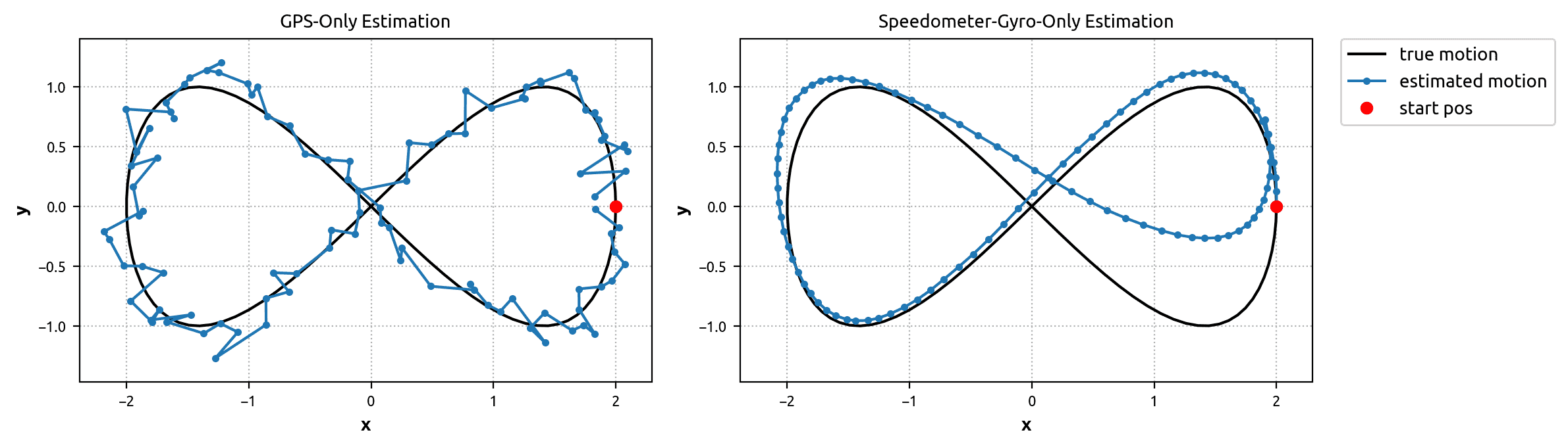
What about using the noisy signals by themselves to estimate the bike’s path? Well, it works up to a point, but has some major defects. For example, relying solely on the GPS signal yields fairly accurate knowledge of the bike’s position at any given time, but the associated velocity and acceleration information is complete garbage (notice how the GPS-only motion estimate below is not smooth). Alternatively, we can use the speedometer and gyroscope signals to estimate the bike’s velocity at any given time, but then the position estimate will diverge as errors accumulate over time.
The Kalman Filter Algorithm
The following is a brief summary of the Kalman Filter Algorithm. For more in-depth explanation of the algorithm, including its motivation and derivation, please see Vaseghi.\(\newcommand{\bm}{\mathbf}\)
The Kalman Equations can be defined as:
where
- \(\bm{x}(t_m)\) is the state vector at time \(t_m\) (e.g., the bike’s position, velocity, acceleration, etc.)
- \(\bm{y}(t_m)\) is the observation vector at time \(t_m\) (e.g., the bike’s sensor measurements)
- \(\bm{A}\) is the transition matrix that relates the state at time \(t_{m-1}\) to the state at time \(t_m\)
- \(\bm{e}(t_m)\) is a Gaussian noise vector representing state transition error; \(\bm{e}\) has a covariance matrix \(\bm{Q}\)
- \(\bm{H}\) is the “channel distortion” matrix that relates the state to the observations at time \(t_m\)
- \(\bm{n}(t_m)\) is a Gaussian noise vector representing the measurement error; \(\bm{n}\) has a covariance matrix \(\bm{R}\)
Additionally, we define:
- \(\bm{\hat{x}}(t_m\mid t_{m-1})\) is the model prediction of the state vector at time \(t_m\) given the previous state
- \(\bm{\hat{x}}(t_m)\) is the estimation of the state vector at time \(t_m\) after observation assimilation
- \(\bm{P}(t_m\mid t_{m-1})\) is the error covariance matrix of the model prediction
- \(\bm{P}(t_m)\) is the error covariance matrix of the estimation
- \(\bm{K}(t_m)\) is the Kalman Gain vector
The Kalman Filter Algorithm requires the following as input:
- Definitions for the \(\bm{A}\), \(\bm{Q}\), \(\bm{H}\), and \(\bm{R}\) matrices
- Best guess initial values for \(\bm{\hat{x}}(t_0\mid t_{-1})\) and \(\bm{P}(t_0\mid t_{-1})\)
- The observation vector \(\bm{y}(t_m)\) for each time-step
For each time-step in the Algorithm, there are two stages. The first stage is the “prediction” stage where we use the model to predict the current state from the previous state. The second is the “estimation” stage where we enhance our prediction with the latest observation data. The \(\bm{\hat{x}}\) and \(\bm{P}\) values at each iteration are calculated thus:
Prediction Stage:
Estimation Stage:
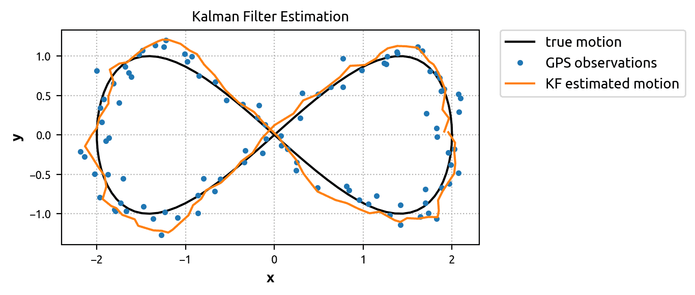
Example 1: GPS Assimilation with the Kalman Filter
This post splits the bike scenario into two Kalman Filter examples. In the first example, we ignore the speedometer and gyroscope sensors completely and only use the GPS sensor to inform our predictive model. The state and observation vectors become:
The first step is to construct our \(\bm{A}\), \(\bm{Q}\), \(\bm{H}\), and \(\bm{R}\) matrices. We’ve already defined our Newtonian predictive model, so we just need to convert it to matrix format to get \(\bm{A}\). Notice how \(\bm{A}\bm{x}(t_{m-1})\) yields a prediction of \(\bm{x}(t_m)\).
A = np.array([[1, dt, (dt**2)/2, 0, 0, 0],[0, 1, dt, 0, 0, 0],[0, 0, 1, 0, 0, 0],[0, 0, 0, 1, dt, (dt**2)/2],[0, 0, 0, 0, 1, dt],[0, 0, 0, 0, 0, 1],])
| 0 | 1 | 2 | 3 | 4 | 5 | |
|---|---|---|---|---|---|---|
| 0 | 1.0 | 0.063467 | 0.002014 | 0.0 | 0.000000 | 0.000000 |
| 1 | 0.0 | 1.000000 | 0.063467 | 0.0 | 0.000000 | 0.000000 |
| 2 | 0.0 | 0.000000 | 1.000000 | 0.0 | 0.000000 | 0.000000 |
| 3 | 0.0 | 0.000000 | 0.000000 | 1.0 | 0.063467 | 0.002014 |
| 4 | 0.0 | 0.000000 | 0.000000 | 0.0 | 1.000000 | 0.063467 |
| 5 | 0.0 | 0.000000 | 0.000000 | 0.0 | 0.000000 | 1.000000 |
To construct \(\bm{Q}\), the error covariance matrix of \(\bm{e}\), we treat the 3rd derivatives of the bike’s \(x\) and \(y\) positions as zero-mean random variables with known variances, \(\sigma_{Jx}^2\) and \(\sigma_{Jy}^2\).
Q1 = np.array([(dt**3)/6, (dt**2)/2, dt, 0, 0, 0])Q1 = np.expand_dims(Q1, 1)Q2 = np.array([0, 0, 0, (dt**3)/6, (dt**2)/2, dt])Q2 = np.expand_dims(Q2, 1)j_var = max(np.var(d3xdt3), np.var(d3ydt3))Q = j_var * (Q1 @ Q1.T + Q2 @ Q2.T)
| 0 | 1 | 2 | 3 | 4 | 5 | |
|---|---|---|---|---|---|---|
| 0 | 5.866119e-08 | 0.000003 | 0.000087 | 0.000000e+00 | 0.000000 | 0.000000 |
| 1 | 2.772857e-06 | 0.000131 | 0.004130 | 0.000000e+00 | 0.000000 | 0.000000 |
| 2 | 8.738015e-05 | 0.004130 | 0.130159 | 0.000000e+00 | 0.000000 | 0.000000 |
| 3 | 0.000000e+00 | 0.000000 | 0.000000 | 5.866119e-08 | 0.000003 | 0.000087 |
| 4 | 0.000000e+00 | 0.000000 | 0.000000 | 2.772857e-06 | 0.000131 | 0.004130 |
| 5 | 0.000000e+00 | 0.000000 | 0.000000 | 8.738015e-05 | 0.004130 | 0.130159 |
Since the GPS device measures the \(x\) and \(y\) positions of the bike directly, the \(\bm{H}\) matrix is easy to construct. It simply filters the state vector to produce an observation vector with \(x_{\text{gps}}\) and \(y_{\text{gps}}\) values only.
H = np.array([[1, 0, 0, 0, 0, 0],[0, 0, 0, 1, 0, 0],])
| 0 | 1 | 2 | 3 | 4 | 5 | |
|---|---|---|---|---|---|---|
| 0 | 1 | 0 | 0 | 0 | 0 | 0 |
| 1 | 0 | 0 | 0 | 1 | 0 | 0 |
\(\bm{R}\), the error covariance matrix of \(\bm{n}\), is known a priori to be a square matrix with the GPS error variances on its diagonal.
R = diag(np.array([gps_sig**2, gps_sig**2]))
| 0 | 1 | |
|---|---|---|
| 0 | 0.01 | 0.00 |
| 1 | 0.00 | 0.01 |
All that’s left to do before applying the Kalman Filter Algorithm is to make best-guesses for the system’s initial state. To keep things simple, we’ll assume that we know the bike’s starting state vector.
x_init = np.array([x[0], dxdt[0], d2xdt2[0], y[0], dydt[0], d2ydt2[0]])P_init = 0.01 * np.eye(len(x_init)) # small initial prediction error
Finally we can apply the the Kalman Filter Algorithm!
# create an observation vector of noisy GPS signalsobservations = np.array([x_gps, y_gps]).T# matrix dimensionsnx = Q.shape[0]ny = R.shape[0]nt = observations.shape[0]# allocate identity matrix for re-useInx = np.eye(nx)# allocate result matricesx_pred = np.zeros((nt, nx)) # prediction of state vectorP_pred = np.zeros((nt, nx, nx)) # prediction error covariance matrixx_est = np.zeros((nt, nx)) # estimation of state vectorP_est = np.zeros((nt, nx, nx)) # estimation error covariance matrixK = np.zeros((nt, nx, ny)) # Kalman Gain# set initial predictionx_pred[0] = x_initP_pred[0] = P_init# for each time-step...for i in range(nt):# prediction stageif i > 0:x_pred[i] = A @ x_est[i-1]P_pred[i] = A @ P_est[i-1] @ A.T + Q# estimation stagey_obs = observations[i]K[i] = P_pred[i] @ H.T @ inv((H @ P_pred[i] @ H.T) + R)x_est[i] = x_pred[i] + K[i] @ (y_obs - H @ x_pred[i])P_est[i] = (Inx - K[i] @ H) @ P_pred[i]
By plotting the \(x\) and \(y\) position estimations (x_est[:, 0] and x_est[:, 3]), we can see that the KF did reasonably well.
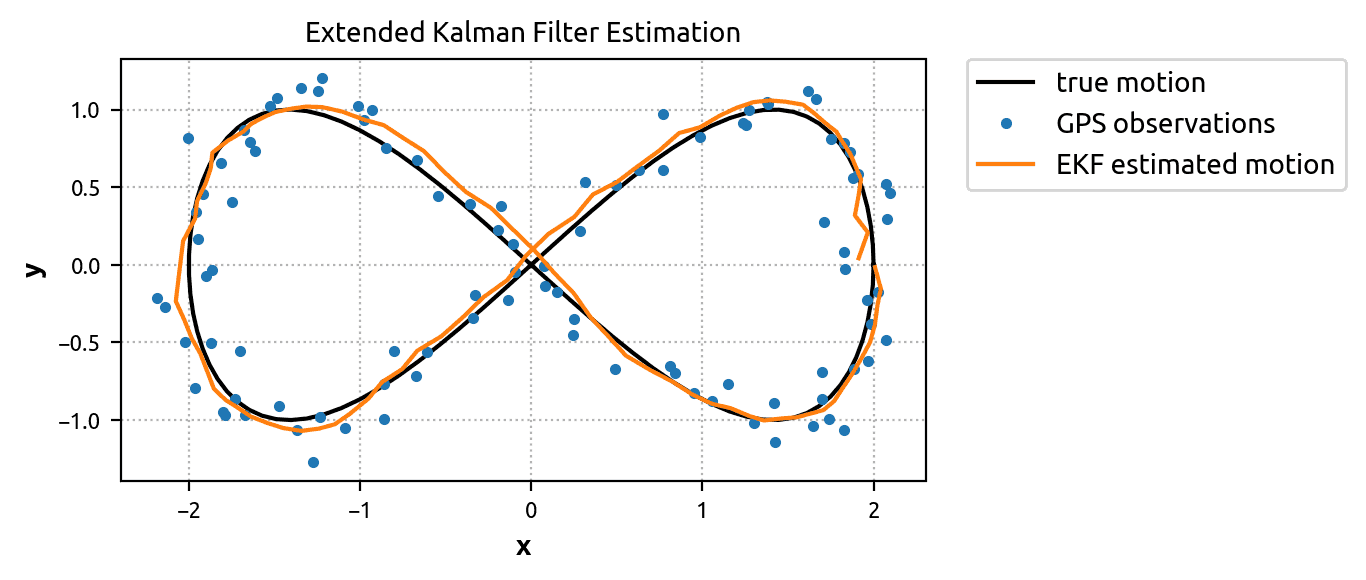
Example 2: Use the Extended Kalman Filter to Assimilate All Sensors
One problem with the normal Kalman Filter is that it only works for models with purely linear relationships. It was fine for the GPS-only example above, but as soon as we try to assimilate data from the other two sensors, the method falls apart. Why? Because the speed and angular speed measurements (\(s\) and \(\omega\)) have non-linear relationships with the bike state vector. As a result, we’re unable to construct a single \(\bm{H}\) matrix that relates state to observation space. Instead, we must work with a non-linear function that relates \(\bm{x}(t_n)\) to \(\bm{y}(t_n)\).
The general (extended) form of the Kalman Equations can be defined:
where \(f\) is a known non-linear model of state transition dynamics and \(h\) is a known non-linear function relating the state to observations. In our case, the transition dynamics remain linear, so we can safely omit \(f\) and continue to use the transition matrix \(\bm{A}\).
However, since we want to use all three sensors, we need to define \(h\) such that it relates the bike state (position, velocity, and acceleration) to observations:
Equipped with the vector function \(h\), the Extended Kalman Filter approximates the \(\bm{H}\) matrix at each time-step by computing the Jacobian at the predicted state vector:
The Python code below defines methods to compute \(h\) and \(\nabla h\) at a state vector for our bike scenario.
def eval_h(x_pred):# expand prediction of state vectorpx, vx, ax, py, vy, ay = x_pred# compute angular velw = (vx*ay - vy*ax) / (vx**2 + vy**2)# compute speeds = sqrt(vx**2 + vy**2)return np.array([px, py, w, s])def eval_H(x_pred):# expand prediction of state vectorpx, vx, ax, py, vy, ay = x_predV2 = vx**2 + vy**2# angular vel partial derivsdwdvx = (V2*ay - 2*vx*(vx*ay-vy*ax)) / (V2**2)dwdax = -vy / V2dwdvy = (-V2*ax - 2*vy*(vx*ay-vy*ax)) / (V2**2)dwday = vx / V2# speed partial derivsdsdvx = vx / sqrt(V2)dsdvy = vy / sqrt(V2)return np.array([[1, 0, 0, 0, 0, 0],[0, 0, 0, 1, 0, 0],[0, dwdvx, dwdax, 0, dwdvy, dwday],[0, dsdvx, 0, 0, dsdvy, 0],])
Other than the modification to \(\bm{H}\), the KF and EKF execute in the same way. One other difference worth noting is that, during the estimation stage, we use \(h\) to evaluate the error between the observation and the predicted observation, not \(\bm{H}\):
Now let’s apply the Extended Kalman Filter Algorithm to assimilate the GPS, speedometer, and gyroscope signals with our predictive model!
# redefine R to include speedometer and gyro variancesR = diag(np.array([gps_sig**2, gps_sig**2, omega_sig**2, speed_sig**2]))
| 0 | 1 | 2 | 3 | |
|---|---|---|---|---|
| 0 | 0.01 | 0.00 | 0.00 | 0.00 |
| 1 | 0.00 | 0.01 | 0.00 | 0.00 |
| 2 | 0.00 | 0.00 | 0.09 | 0.00 |
| 3 | 0.00 | 0.00 | 0.00 | 0.01 |
# create an observation vector of all noisy signalsobservations = np.array([x_gps, y_gps, omega_sens, speed_sens]).T# matrix dimensionsnx = Q.shape[0]ny = R.shape[0]nt = observations.shape[0]# allocate identity matrix for re-useInx = np.eye(nx)# allocate result matricesx_pred = np.zeros((nt, nx)) # prediction of state vectorP_pred = np.zeros((nt, nx, nx)) # prediction error covariance matrixx_est = np.zeros((nt, nx)) # estimation of state vectorP_est = np.zeros((nt, nx, nx)) # estimation error covariance matrixK = np.zeros((nt, nx, ny)) # Kalman Gain# set initial predictionx_pred[0] = x_initP_pred[0] = P_init# for each time-step...for i in range(nt):# prediction stageif i > 0:x_pred[i] = A @ x_est[i-1]P_pred[i] = A @ P_est[i-1] @ A.T + Q# estimation stagey_obs = observations[i]y_pred = eval_h(x_pred[i])H_pred = eval_H(x_pred[i])K[i] = P_pred[i] @ H_pred.T @ inv((H_pred @ P_pred[i] @ H_pred.T) + R)x_est[i] = x_pred[i] + K[i] @ (y_obs - y_pred)P_est[i] = (Inx - K[i] @ H_pred) @ P_pred[i]
By plotting the \(x\) and \(y\) position estimations (x_est[:, 0] and x_est[:, 3]), we can see that the EKF did even better than the KF. The estimated motion is very smooth and fits the true solution tightly. Clearly the extra information from the speedometer and gyroscope is useful. It’s just a matter of assimilating it with the predictive model in the right way!
Conclusion
I hope you found these two examples informative. Personally, I found it very instructive working through the process of mocking up the bike scenario and then applying the KF and EKF to the artificial data. Conceivably, one could test this exact procedure out in the real world by attaching GPS, speedometer, and gyroscope sensors to their bike and taking a ride around the park. However, before doing that, one should recognize the many assumptions and simplifications made in this scenario — not the least of which is that the \(z\)-axis is completely ignored!
It is left to the reader to take the scenario even further by investigating the other statistical quantities generated by the KF and EKF. For example, what is the Kalman Gain, K, and how does one interpret it? How do the predicted state vectors in x_pred compare to the estimated state vectors in x_est? How does one use the P_pred and P_est matrices?
One thing I might like to do is apply the Unscented Kalman Filter (UKF) to the scenario to see how it manages. But that’s a task for another day.
References
- Vaseghi, Saeed. Advanced Digital Signal Processing and Noise Reduction. Wiley, 2008.
- Kutz, J. Nathan. Data-driven modeling & scientific computation: methods for complex systems & big data. OUP Oxford, 2013.
GET IN TOUCH
Have a project in mind?
Reach out directly to hello@humaticlabs.com or use the contact form.