Dynamic Mode Decomposition in Python

The Dynamic Mode Decomposition (DMD) is a relatively recent mathematical innovation that, among other things, allows us to solve or approximate dynamical systems in terms of coherent structures that grow, decay, and/ or oscillate in time. We refer to the coherent structures as DMD modes. Each DMD mode has corresponding time dynamics defined in terms of a single eigenvalue.

In other words, the DMD converts a dynamical system into a superposition of modes whose dynamics are governed by eigenvalues.

Amazingly, although the mathematical procedure for identifying the DMD modes and eigenvalues is purely linear, the system itself can be nonlinear! I won’t go into it here but there are sound theoretical underpinnings for the claim that a nonlinear system can be described by a set of mode and eigenvalue pairs. Read up on the Koopman operator and the DMD’s connection to it for more information (see references at bottom).

Not only is the DMD a useful diagnostic tool for analyzing the inner workings of a system, but it can also be used to predict the future state of the system. All that is needed are the modes and the eigenvalues. With very little effort, the modes and eigenvalues can be combined to produce a function that approximates the system state at any moment in time.

In this post, I start by briefly introducing the mathematical theory of the DMD. Then I go over a number of examples with annotated Python code. The examples are just toy problems, but they succeed in illustrating how to use the DMD in several different situations, including:

• Given: a 1-dimensional scalar function evolving in time.
• Given: a set of trajectories in 3 dimensions produced by an unknown vector field.
• Given: a set of 3-dimensional vectors sampled from an unknown vector field.
• Given: a 2-dimensional scalar function in spherical coordinates evolving in time.

It is important to fully understand the limitations of any modeling strategy. Thus, I also talk a bit about when and how the DMD can fail. Finally, I conclude the post with a mention of notable extensions to the DMD and a summary.

Formal Definition

Consider a set of \(n\) data pairs

in which each \(x_i\) and \(y_i\) is a column vector of size \(m\). We now define two \(m\times n\) matrices:

If we define an operator \(A\) as

where \(X^\dagger\) is the pseudo-inverse of \(X\), then the Dynamic Mode Decomposition of the pair \((X,Y)\) is given by the eigendecomposition of \(A\). That is, the DMD modes and eigenvalues are eigenvectors and eigenvalues of \(A\).

The definition above, from Tu et al., is known as the exact DMD. It is currently the most general definition and can be applied to any dataset that satisfies the given requirements. In this post, we are mostly interested in the cases where \(A\) satisfies (perhaps approximately) the equation \(y_i=Ax_i\) for all \(i\). Or, more precisely:

Clearly, \(X\) is a set of inputs vectors and \(Y\) is the corresponding set of output vectors. This particular interpretation of the DMD is extremely powerful, as it provides a convenient method for analyzing (and predicting) dynamical systems for which the governing equations are unknown. More on dynamical systems shortly.

There are a number of theorems that go along with this definition of the DMD. One of the more useful theorems states that \(Y=AX\) exactly if and only if \(X\) and \(Y\) are linearly consistent (i.e., whenever \(Xv=0\) for some vector \(v\), then \(Yv=0\) too). Linear consistency is relatively straightforward to test, as we shall see. That being said, linear consistency is not a mandatory prerequisite for using the DMD. Even if the DMD solution for \(A\) doesn’t exactly satisfy the equation \(Y=AX\), it is still a least-squares solution, minimizing error in an \(L^2\) sense.

DMD Algorithm

At first glance, the task of finding the eigendecomposition of \(A=YX^\dagger\) doesn’t appear to be too big of a deal. Indeed, when \(X\) and \(Y\) are reasonably sized, a couple calls to the pinv and eig methods from Numpy or MATLAB will do the trick. The problem comes when \(A\) is truly large. Notice that \(A\) is \(m\times m\), so when \(m\) (the number of signals in each time sample) is very large, finding the eigendecomposition can become unwieldy.

Fortunately, the problem can be broken down into smaller pieces with the help of the exact DMD algorithm.

1. Compute the SVD of \(X\), optionally performing a low-rank truncation at the same time:

2. Compute \(\tilde A\), the projection of the full matrix \(A\) onto \(U\):

3. Compute the eigenvalues \(\lambda_i\) and eigenvectors \(w_i\) of \(\tilde A\):

4. Reconstruct the eigendecomposition of \(A\) from \(W\) and \(\Lambda\). The eigenvalues for \(A\) are equivalent to those of \(\tilde A\). The eigenvectors of \(A\) are given by the columns of \(\Phi\):

A more in-depth explanations of the algorithm’s derivation can be found in the references. It also might be of theoretical interest to note that \(\Phi=UW\) is an alternate derivation of \(\Phi\) referred to as the projected DMD modes. In this post, I only use exact DMD modes.

Now let’s go through the algorithm step-by-step in Python. Start by installing and importing all necessary packages.

import numpy as np
import matplotlib as mpl
import matplotlib.pyplot as plt
from mpl_toolkits.mplot3d import Axes3D
from numpy import dot, multiply, diag, power
from numpy import pi, exp, sin, cos, cosh, tanh, real, imag
from numpy.linalg import inv, eig, pinv
from scipy.linalg import svd, svdvals
from scipy.integrate import odeint, ode, complex_ode
from warnings import warn

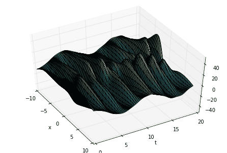
Let’s generate some play data. Keep in mind that in practice, one doesn’t necessarily know the governing equations for a data. Here we’re just inventing some equations to create a dataset. Forget they ever existed once the data has been generated.

# define time and space domains
x = np.linspace(-10, 10, 100)
t = np.linspace(0, 6*pi, 80)
dt = t[2] - t[1]
Xm,Tm = np.meshgrid(x, t)

# create three spatiotemporal patterns
f1 = multiply(20-0.2*power(Xm, 2), exp((2.3j)*Tm))
f2 = multiply(Xm, exp(0.6j*Tm))
f3 = multiply(5*multiply(1/cosh(Xm/2), tanh(Xm/2)), 2*exp((0.1+2.8j)*Tm))

# combine signals and make data matrix
D = (f1 + f2 + f3).T

# create DMD input-output matrices
X = D[:,:-1]
Y = D[:,1:]

Now compute the SVD of \(X\). The first variable of major interest is \(\Sigma\), the singular values of \(X\). Taking the SVD of \(X\) allows us to extract its “high-energy” modes and reduce the dimensionality of the system a la Proper Orthogonal Decomposition (POD). Looking at the singular values informs our decision of how many modes to truncate.

# SVD of input matrix
U2,Sig2,Vh2 = svd(X, False)

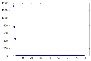
Given the singular values shown above, we conclude that the data has three modes of any significant interest. Therefore, we truncate the SVD to only include those modes. Then we build \(\tilde A\) and find its eigendecomposition.

# rank-3 truncation
r = 3
U = U2[:,:r]
Sig = diag(Sig2)[:r,:r]
V = Vh2.conj().T[:,:r]

# build A tilde
Atil = dot(dot(dot(U.conj().T, Y), V), inv(Sig))
mu,W = eig(Atil)

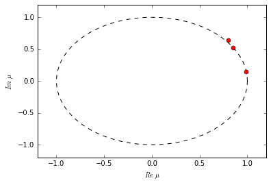
Each eigenvalue in \(\Lambda\) tells us something about the dynamic behavior of its corresponding DMD mode. Its exact interpretation depends on the nature of the relationship between \(X\) and \(Y\). In the case of difference equations we can make a number of conclusions. If the eigenvalue has a non-zero imaginary part, then there is oscillation in the corresponding DMD mode. If the eigenvalue is inside the unit circle, then the mode is decaying; if the eigenvalue is outside, then the mode is growing. If the eigenvalue falls exactly on the unit circle, then the mode neither grows nor decays.

Now build the exact DMD modes.

# build DMD modes
Phi = dot(dot(dot(Y, V), inv(Sig)), W)

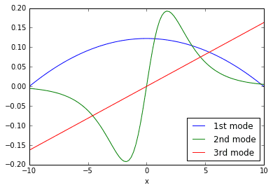
The columns of \(\Phi\) are the DMD modes plotted above. They are the coherent structures that grow/ decay/ oscillate in the system according to different time dynamics. Compare the curves in the plot above with the rolling, evolving shapes seen in the original 3D surface plot. You should notice similarities.

This is where the DMD algorithm technically ends. Equipped with the eigendecomposition of \(A\) and a basic understanding of the nature of the system \(Y=AX\), it is possible to construct a matrix \(\Psi\) corresponding to the system’s time evolution. To fully understand the code below, study the function \(x(t)\) for difference equations in the next section.

# compute time evolution
b = dot(pinv(Phi), X[:,0])
Psi = np.zeros([r, len(t)], dtype='complex')
for i,_t in enumerate(t):
    Psi[:,i] = multiply(power(mu, _t/dt), b)

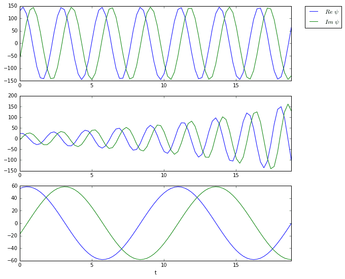
The three plots above are the time dynamics of the three DMD modes. Notice how all three are oscillating. Furthermore, the second mode appears to grow exponentially, which is confirmed by the eigenvalue plot.

If you wish to construct an approximation to the original data matrix, simply multiply \(\Phi\) and \(\Psi\). The original and the approximation match up exactly in this particular case.

# compute DMD reconstruction
D2 = dot(Phi, Psi)
np.allclose(D, D2) # True

Dynamical Systems

I only consider two interpretations of the equation \(Y=AX\) in this post. The first interpretation is where \(A\) defines a difference equation:

In this case, the operator \(A\) takes a dynamical system state \(x_i\) one step forward in time. Let’s say that we have a time series \(D\):

where \(x_i\) is a column vector defining the system’s \(m\)-dimensional state at time-step \(i\). Then, we can define \(X\) and \(Y\) such that:

In this way, each pair of columns vectors from \(X\) and \(Y\) correspond to a single iteration of the difference equation, and in general:

Using the DMD, we find the eigendecomposition of \(A\Phi=\Phi\Lambda\). With the DMD modes and eigenvalues in hand, we can easily convert \(Y=AX\) into a function defined in terms of discrete time iterations \(k\) with time-step \(\Delta t\):

The corresponding function in continuous time \(t\) would be

What is truly amazing is that we have just defined explicit functions in time using nothing but data! This is a good example of equation-free modeling.

The second interpretation of \(Y=AX\) considered in this post is where \(A\) defines a system of differential equations:

In this case, the operator \(A\) computes the first derivative with respect to time of a vector \(x_i\). Our matrices \(X\) and \(Y\) would then consist of \(n\) samples of a vector field: the \(i\)-th column of \(X\) is a position vector \(x_i\); the \(i\)-th column of \(Y\) is a velocity vector \(\dot x_i\).

After computing the DMD, the function in time is very similar to before (i.e., of the difference equation). If \(x(0)\) is an arbitrary initial condition and \(t\) is continuous time, then

Examples

Here are a few of examples of how to use the DMD with different types of experimental data. For convenience, I condense the DMD code into a single method and define some helper methods to check linear consistency and confirm my solutions.

def nullspace(A, atol=1e-13, rtol=0):
    # from http://scipy-cookbook.readthedocs.io/items/RankNullspace.html
    A = np.atleast_2d(A)
    u, s, vh = svd(A)
    tol = max(atol, rtol * s[0])
    nnz = (s >= tol).sum()
    ns = vh[nnz:].conj().T
    return ns

def check_linear_consistency(X, Y, show_warning=True):
    # tests linear consistency of two matrices (i.e., whenever Xc=0, then Yc=0)
    A = dot(Y, nullspace(X))
    total = A.shape[1]
    z = np.zeros([total, 1])
    fails = 0
    for i in range(total):
        if not np.allclose(z, A[:,i]):
            fails += 1
    if fails > 0 and show_warning:
        warn('linear consistency check failed {} out of {}'.format(fails, total))
    return fails, total

def dmd(X, Y, truncate=None):
    U2,Sig2,Vh2 = svd(X, False) # SVD of input matrix
    r = len(Sig2) if truncate is None else truncate # rank truncation
    U = U2[:,:r]
    Sig = diag(Sig2)[:r,:r]
    V = Vh2.conj().T[:,:r]
    Atil = dot(dot(dot(U.conj().T, Y), V), inv(Sig)) # build A tilde
    mu,W = eig(Atil)
    Phi = dot(dot(dot(Y, V), inv(Sig)), W) # build DMD modes
    return mu, Phi

def check_dmd_result(X, Y, mu, Phi, show_warning=True):
    b = np.allclose(Y, dot(dot(dot(Phi, diag(mu)), pinv(Phi)), X))
    if not b and show_warning:
        warn('dmd result does not satisfy Y=AX')

3D Vector Field: Difference Equation

In this first example, we are given a set of trajectories in 3 dimensions produced by an vector field. I used the following system of differential equations to produce the trajectories.

Watch the video below for an animation of the dynamic behavior.

You can generate a dataset with the following code. Basically, it randomly chooses a set of initial points and simulates each of them forward in time. Then it concatenates all of the individual trajectories together to produce \(X\) and \(Y\) matrices.

# convenience method for integrating
def integrate(rhs, tspan, y0):
    
    # empty array to hold solution
    y0 = np.asarray(y0) # force to numpy array
    Y = np.empty((len(y0), tspan.size), dtype=y0.dtype)
    Y[:, 0] = y0

    # auto-detect complex systems
    _ode = complex_ode if np.iscomplexobj(y0) else ode
    
    # create explicit Runge-Kutta integrator of order (4)5
    r = _ode(rhs).set_integrator('dopri5')
    r.set_initial_value(Y[:, 0], tspan[0])

    # run the integration
    for i, t in enumerate(tspan):
        if not r.successful():
            break
        if i == 0:
            continue # skip the initial position
        r.integrate(t)
        Y[:, i] = r.y

    # return solution
    return Y

# the right-hand side of our ODE
def saddle_focus(t, y, rho = 1, omega = 1, gamma = 1):

    return dot(np.array([
                [-rho, -omega, 0],
                [omega, -rho, 0],
                [0, 0, gamma]
            ]), y)

# generate data
dt = 0.01
tspan = np.arange(0, 50, dt)
X = np.zeros([3, 0])
Y = np.zeros([3, 0])
z_cutoff = 15 # to truncate the trajectory if it gets too large in z
for i in range(20):
    theta0 = 2*pi*np.random.rand()
    x0 = 3*cos(theta0)
    y0 = 3*sin(theta0)
    z0 = np.random.randn()
    D = integrate(saddle_focus, tspan, [x0, y0, z0])
    D = D[:,np.abs(D[2,:]) < z_cutoff]
    X = np.concatenate([X, D[:,:-1]], axis=1)
    Y = np.concatenate([Y, D[:,1:]], axis=1)
    
check_linear_consistency(X, Y); # raise a warning if not linearly consistent

Now compute the DMD, just like before.

mu,Phi = dmd(X, Y, 3)
check_dmd_result(X, Y, mu, Phi) # raise a warning if Y=AX not satisfied

The DMD computation was successful. Given an initial condition \(x(0)\), you can simulate the solution forward in time with the following code.

# simulate an initial condition forward in time
b = dot(pinv(Phi), np.array([3.45, -0.2, 0.98]).T)
Psi = np.zeros([3, len(tspan)], dtype='complex')
for i,_t in enumerate(tspan):
    Psi[:,i] = multiply(power(mu, _t/dt), b)
Dtil = real(dot(Phi, Psi))

Of course, instead of using the DMD, it probably would have been a lot easier just to compute \(A=YX^\dagger\) directly. We’re only dealing with three spatial dimensions after all. But that would defeat the purpose of the exercise… ;)

3D Vector Field: Differential Equation

This example is very, very similar to the previous example. We shall use the same “mystery” vector field to create the dataset. The only difference is that the following code directly samples the output of the system of differential equations instead of simulating trajectories. In other words, we generate the data by randomly generating a set of position vectors, \(X\), and feeding them into the system to produce velocity vectors, \(Y\).

# randomly generate a set of position vectors
X = np.random.rand(3, 5000) * 10 - 5

# compute the corresponding velocity vectors
Y = saddle_focus(0, X)

# compute the DMD for the "unknown" data
mu,Phi = dmd(X, Y, 3)
check_dmd_result(X, Y, mu, Phi) # raise a warning if Y=AX not satisfied

The decomposition is successful. As extra confirmation, when we examine the eigenvalues, we notice that they are the same eigenvalues as the original system that produced our dataset. There are two oscillating-decaying modes (complex conjugates) and one exponentially growing mode. Watch the video again to witness these exact time dynamics.

Spherical coordinates

This example demonstrates that the spatial dimension of \(X\) and \(Y\) can be defined however we like. Specifically, let’s generate a dataset in spherical coordinates. The modes shall essentially be scalar functions defined in terms of \(\theta\) and \(\phi\). That is:

The mystery dataset is that of a \(r=4\) sphere with five oscillating modes. Watch the video for an animation.

# define time and space domains
q = np.linspace(0, 2 * pi, 40) # theta
p = np.linspace(0, pi, 40) # phi
t = np.linspace(0, 80, 800) # time
dt = t[1] - t[0]
Qm,Pm = np.meshgrid(q, p)

# each column of the dataset is a flattened theta-phi matrix
R = np.zeros([len(q)*len(p), len(t)], dtype='complex') # must be complex
for i in range(len(t)):
    R[:,i] = (
        4 # a stationary mode
        + 0.4 * cos(10 * Qm) * cos(10 * Pm) * exp(t[i] * 3.2j)
        + 0.1 * cos(16 * Qm) * cos(22 * Pm) * exp(t[i] * 5.0j)
        + 0.6 * exp(t[i] * 0.7j)
        + 0.7 * cos(5 * Qm) * exp(t[i] * 1.5j)
        - 0.3 * cos(9 * Pm) * exp(t[i] * 0.3j)
        ).flatten()

# subtract off the mean (approx. 4) to prevent corruption of modes
R -= R.mean()

# extract X,Y matrices
X = R[:,:-1]
Y = R[:,1:]
check_linear_consistency(X, Y)

It is important to note that during the spheroid investigation, I found that the existence of the stationary, non-zero mode (i.e., the constant radius of 4) caused the DMD to fail. One would think that the constant mode would be the easiest mode to identify, but it was not. Instead, the DMD tried to account for the influence of constant mode by injecting it into the other modes, thereby corrupting the results. My conclusion is that, under certain circumstances, the singular value corresponding to the constant mode can shrink so small that the SVD-based DMD misses it completely.

Given that this is a potential problem for some datasets, it is probably a good idea to pre-process your dataset by removing the mean of each signal in the data matrix. While your at it, you could divide each signal by its variance to completely normalize the data.

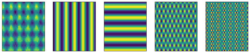
# compute DMD
r = 5
mu,Phi = dmd(X, Y, r)
check_dmd_result(X, Y, mu, Phi)

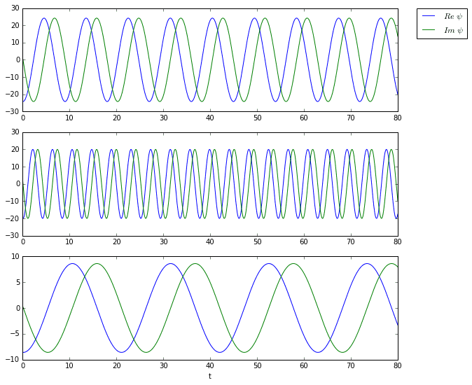
Here are visualizations of the five DMD modes. Each pseudo-color plot represents a different scalar function \(r=f(\theta,\phi)\). Each mode oscillates at some frequency (determined by the eigenvalues) in spherical coordinates.

And here are the time dynamics of the first three modes.

Limitations

The DMD has several known limitations. First of all, it doesn’t handle translational and rotational invariance particularly well. Secondly, it can fail completely when transient time behavior is present. The follow examples illustrate these problems.

Translational Invariance

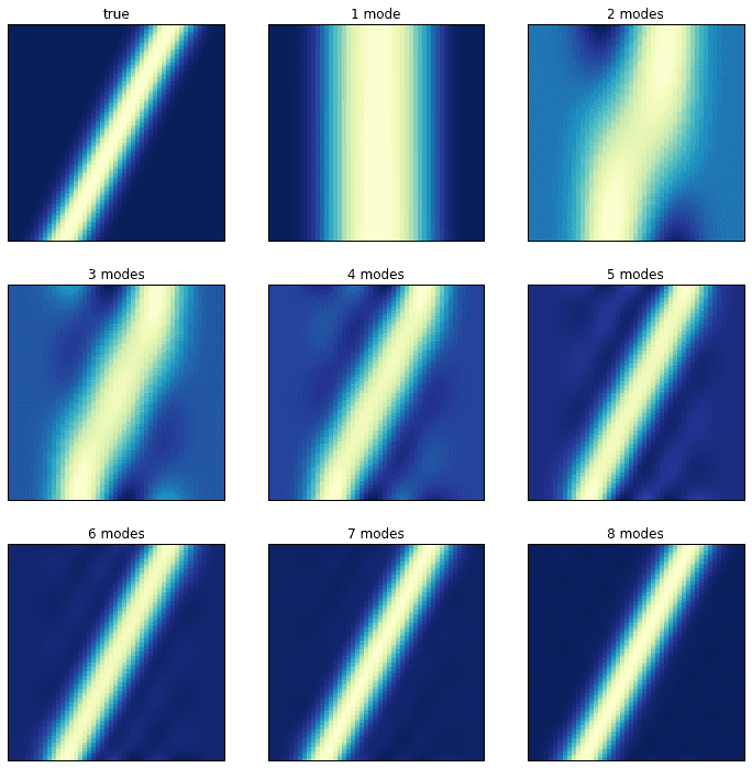
The following dataset is very simple. It consists of a single mode (a Gaussian) translating along the spatial domain as the system evolves. Although one would think that the DMD would handle this cleanly, the opposite happens. Instead of picking up a single, well-defined singular value, the SVD picks up many.

# define time and space domains
x = np.linspace(-10, 10, 50)
t = np.linspace(0, 10, 100)
dt = t[2] - t[1]
Xm,Tm = np.meshgrid(x, t)

# create data with a single mode traveling both spatially and in time
D = exp(-power((Xm-Tm+5)/2, 2))
D = D.T

# extract input-output matrices
X = D[:,:-1]
Y = D[:,1:]
check_linear_consistency(X, Y)

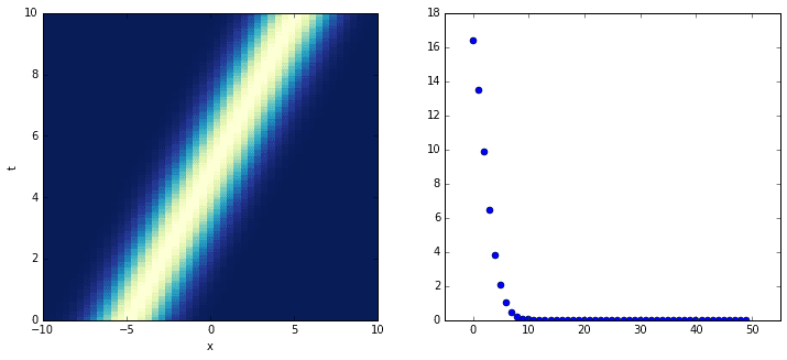
The plot on the left shows the evolution of the system; the plot on the right shows its singular values. It turns out that close to ten DMD modes are needed to correctly approximate the system! Consider the following plots in which the original, true dynamics are compared to the superpositions of an increasing number of modes.

Transient time behavior

In this final example, we look at a dataset containing transient time dynamics. Specifically, the data shows a Gaussian popping in and out of existence. Unfortunately, the DMD cannot accurately decompose this data.

# define time and space domains
x = np.linspace(-10, 10, 50)
t = np.linspace(0, 10, 100)
dt = t[2] - t[1]
Xm,Tm = np.meshgrid(x, t)

# create data with a single transient mode
D = exp(-power((Xm)/4, 2)) * exp(-power((Tm-5)/2, 2))
D = D.astype('complex').T

# extract input-output matrices
X = D[:,:-1]
Y = D[:,1:]
check_linear_consistency(X, Y)

# do dmd
r = 1
mu,Phi = dmd(X, Y, r)
check_dmd_result(X, Y, mu, Phi)

# time evolution
b = dot(pinv(Phi), X[:,0])
Psi = np.zeros([r, len(t)], dtype='complex')
for i,_t in enumerate(t):
    Psi[:,i] = multiply(power(mu, _t/dt), b)

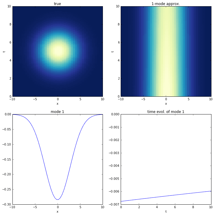
Although the DMD correctly identifies the mode, it fails completely to identify the time-behavior. This is understandable if we consider that the time-behavior of the DMD time series depends on eigenvalues, which are only capable of characterizing combinations of exponential growth (the real part of the eigenvalue) and oscillation (the imaginary part).

The interesting thing about this system is that an ideal decomposition could potentially consist of a superposition of a single mode (as shown in the figure) with various eigenvalues. Imagine the single mode being multiplied by a linear combination of many orthogonal sines and cosines (a Fourier series) that approximates the true time dynamics. Unfortunately, a single application of the SVD-based DMD is incapable of yielding the same DMD mode various times with different eigenvalues.

Furthermore, it is important to note that even if we were able to correctly extract the time behavior as a large set of eigenvalues, the solution’s predictive capabilities would not be reliable without fully understanding the transient behavior itself. Transient behavior, by its very nature, is non-permanent.

The multi-resolution DMD (mrDMD) attempts to alleviate the transient time behavior problem by means of a recursive application of the DMD.

Conclusion

Despite its limitations, the DMD is a very powerful tool for analyzing and predicting dynamical systems. All data scientists from all backgrounds should have a good understanding of the DMD and how to apply it. The purpose of this post is to provide some theory behind the DMD and to provide practical code examples in Python that can be used with real-world data. After studying the formal definition of the DMD, walking through the algorithm step-by-step, and playing with several simple examples of its use — including examples in which it fails — it is my hope that this post has provided you an even clearer understanding of the DMD and how it might be applied in your research or engineering project.

There are many extensions to the DMD. Future work will likely result in posts on some of these extensions, including the multi-resolution DMD (mrDMD) and the sparse DMD (sDMD).

References

1. Kutz, J. Nathan. Data-driven modeling & scientific computation: methods for complex systems & big data. OUP Oxford, 2013.
2. Tu, Jonathan H., et al. “On dynamic mode decomposition: theory and applications.” arXiv preprint arXiv:1312.0041 (2013).
3. Wikipedia contributors. “Composition operator.” Wikipedia, The Free Encyclopedia. Wikipedia, The Free Encyclopedia, 28 Dec. 2015. Web. 24 Jul. 2016.
4. Wikipedia contributors. “Moore–Penrose pseudoinverse.” Wikipedia, The Free Encyclopedia. Wikipedia, The Free Encyclopedia, 12 May. 2016. Web. 24 Jul. 2016.